library(ggtree)
library(ggplot2)
library(dplyr)
#setwd("/home/jhuang/DATA/Data_Ben_Boruta_Analysis/plotTreeHeatmap_ecoli/")
info <- read.csv("isolate_ecoli_.csv", sep="\t", check.names = FALSE)
info$name <- info$Isolate
# make ST discrete
info$ST <- factor(info$ST)
tree <- read.tree("../ecoli_core_gene_tree_1000.raxml.bestTree")
cols <- c("10"="cornflowerblue","38"="darkgreen","46"="seagreen3","69"="tan","88"="red", "131"="navyblue", "156"="gold", "167"="green","216"="orange","405"="pink","410"="purple","1882"="magenta","2450"="brown", "2851"="darksalmon","3570"="chocolate4","4774"="darkkhaki")
# "290"="azure3", "297"="maroon","325"="lightgreen", "454"="blue","487"="cyan", "558"="skyblue2", "766"="blueviolet"
#heatmapData2 <- info %>% select(Isolate, blaCTX.M, blaIMP, blaKPC, blaNDM.1, blaNDM.5, blaOXA.23.like, blaOXA.24.like, blaOXA.48.like, blaOXA.58.like, blaPER.1, blaSHV, blaVEB.1, blaVIM) #ST,
heatmapData2 <- info %>% select(
Isolate,
`blaCTX-M`, blaIMP, blaKPC, `blaNDM-1`, `blaNDM-5`,
`blaOXA-23-like`, `blaOXA-24-like`, `blaOXA-48-like`, `blaOXA-58-like`,
`blaPER-1`, blaSHV, `blaVEB-1`, blaVIM
)
rn <- heatmapData2$Isolate
heatmapData2$Isolate <- NULL
heatmapData2 <- as.data.frame(sapply(heatmapData2, as.character))
rownames(heatmapData2) <- rn
#heatmap.colours <- c("darkred", "darkblue", "darkgreen", "grey")
#names(heatmap.colours) <- c("MT880870","MT880871","MT880872","-")
#heatmap.colours <- c("cornflowerblue","darkgreen","seagreen3","tan","red", "navyblue", "gold", "green","orange","pink","purple","magenta","brown", "darksalmon","chocolate4","darkkhaki", "azure3", "maroon","lightgreen", "blue","cyan", "skyblue2", "blueviolet", "darkred", "darkblue", "darkgreen", "grey")
#names(heatmap.colours) <- c("2","5","7","9","14", "17","23", "35","59","73", "81","86","87","89","130","190","290", "297","325", "454","487","558","766", "MT880870","MT880871","MT880872","-")
#heatmap.colours <- c("cornflowerblue","darkgreen","seagreen3","tan","red", "navyblue", "purple", "green","cyan", "darkred", "darkblue", "darkgreen", "grey", "darkgreen", "grey")
#names(heatmap.colours) <- c("SCCmec_type_II(2A)", "SCCmec_type_III(3A)", "SCCmec_type_III(3A) and SCCmec_type_VIII(4A)", "SCCmec_type_IV(2B)", "SCCmec_type_IV(2B&5)", "SCCmec_type_IV(2B) and SCCmec_type_VI(4B)", "SCCmec_type_IVa(2B)", "SCCmec_type_IVb(2B)", "SCCmec_type_IVg(2B)", "I", "II", "III", "none", "+","-")
heatmap.colours <- c("darkgreen", "grey")
names(heatmap.colours) <- c("+","-")
#mydat$Regulation <- factor(mydat$Regulation, levels=c("up","down"))
#circular
p <- ggtree(tree, layout='circular', branch.length='none') %<+% info + geom_tippoint(aes(color=ST)) + scale_color_manual(values=cols) + geom_tiplab2(aes(label=name), offset=1)
png("ggtree.png", width=1260, height=1260)
#svg("ggtree.svg", width=1260, height=1260)
p
dev.off()
#gheatmap(p, heatmapData2, width=0.1, colnames_position="top", colnames_angle=90, colnames_offset_y = 0.1, hjust=0.5, font.size=4, offset = 5) + scale_fill_manual(values=heatmap.colours) + theme(legend.text = element_text(size = 14)) + theme(legend.title = element_text(size = 14)) + guides(fill=guide_legend(title=""), color = guide_legend(override.aes = list(size = 5)))
png("ggtree_and_gheatmap_mibi_selected_genes.png", width=1590, height=1300)
#svg("ggtree_and_gheatmap_mibi_selected_genes.svg", width=17, height=15)
gheatmap(p, heatmapData2, width=2, colnames_position="top", colnames_angle=90, colnames_offset_y = 2.0, hjust=0.7, font.size=4, offset = 8) + scale_fill_manual(values=heatmap.colours) + theme(legend.text = element_text(size = 16)) + theme(legend.title = element_text(size = 16)) + guides(fill=guide_legend(title=""), color = guide_legend(override.aes = list(size = 5)))
dev.off()
# ---------
# 1) Optional: shrink tree to create more outer space (keeps relative scale)
tree_small <- tree
tree_small$edge.length <- tree_small$edge.length * 0.4 # try 0.3–0.5
# 2) Height after shrinking
ht <- max(ape::node.depth.edgelength(tree_small))
# 3) Base tree
info$ST <- factor(info$ST)
p <- ggtree(tree_small, layout = "circular", open.angle = 20) %<+% info +
geom_tippoint(aes(color = ST), size = 1.4) +
geom_tiplab2(aes(label = name), size = 1.4, offset = 0.02 * ht) +
scale_color_manual(values = cols)
# 4) Reserve room outside the tips
off <- 0.30 * ht # gap
wid <- 2.80 * ht # ring thickness
mar <- 0.25 * ht
p_wide <- p + xlim(0, ht + off + wid + mar)
# 5) Ensure discrete values are factors and keep both levels
heatmapData2[] <- lapply(heatmapData2, function(x) factor(x, levels = c("+","-")))
# 6) Draw the heatmap
png("ggtree_and_gheatmap_readable.png", width = 3600, height = 3200, res = 350)
gheatmap(
p_wide, heatmapData2,
offset = off,
width = wid,
color = "white", # borders between tiles
colnames = TRUE,
colnames_position = "top",
colnames_angle = 0,
colnames_offset_y = 0.04 * ht,
hjust = 0.5,
font.size = 7
) +
scale_fill_manual(values = c("+"="darkgreen", "-"="grey"), drop = FALSE) +
guides(
fill = guide_legend(title = "", override.aes = list(size = 4)),
color = guide_legend(override.aes = list(size = 3))
)
dev.off()
#-------------- plot with true scale -------------
# tree height (root → farthest tip)
ht <- max(ape::node.depth.edgelength(tree))
# circular tree with a small opening and compact labels
p <- ggtree(tree, layout = "circular", open.angle = 20) %<+% info +
geom_tippoint(aes(color = ST), size = 1.8, alpha = 0.9) +
geom_tiplab2(aes(label = name), size = 2.2, offset = 0.06 * ht) +
scale_color_manual(values = cols) +
theme(legend.title = element_text(size = 12),
legend.text = element_text(size = 10))
# higher-DPI export so small cells look crisp
png("ggtree_true_scale.png", width = 2400, height = 2400, res = 300)
p
dev.off()
# --- Heatmap: push it further out and make it wider ---
#svg("ggtree_and_gheatmap_mibi_selected_genes_true_scale.svg",
# width = 32, height = 28)
png("ggtree_and_gheatmap_mibi_selected_genes_true_scale.png",
width = 2000, height = 1750, res = 200)
gheatmap(
p, heatmapData2,
offset = 0.24 * ht, # farther from tips (was 0.08*ht)
width = 20.0 * ht, # much wider ring (was 0.35*ht)
color = "white", # thin tile borders help readability
colnames_position = "top",
colnames_angle = 90, # keep column labels horizontal to save space
colnames_offset_y = 0.08 * ht,
hjust = 0.1,
font.size = 2.6 # bigger column label font
) +
scale_fill_manual(values = heatmap.colours) +
guides(fill = guide_legend(title = "", override.aes = list(size = 4)),
color = guide_legend(override.aes = list(size = 3))) +
theme(legend.position = "right",
legend.title = element_text(size = 10),
legend.text = element_text(size = 8))
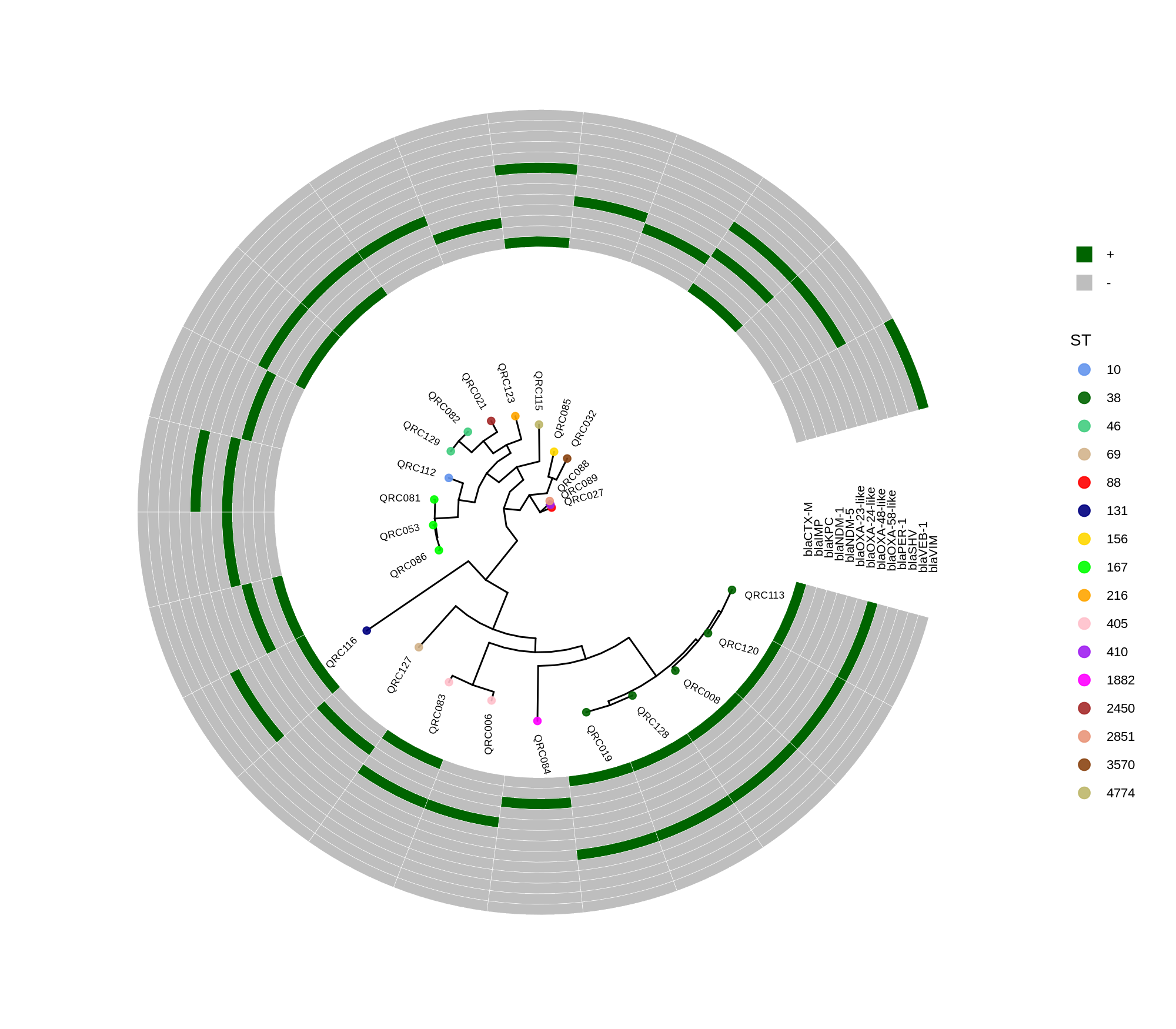
dev.off()This R script visualizes a phylogenetic tree of E. coli isolates using the ggtree and ggplot2 packages, annotated with sequence type (ST) colors and a heatmap showing the presence or absence of antimicrobial resistance genes. It creates several versions of the circular tree figure to adjust scaling and readability.
Key Steps
- Load libraries and data
The code imports
ggtree,ggplot2, anddplyr, reads isolate metadata (isolate_ecoli_.csv), and loads a phylogenetic tree file (ecoli_core_gene_tree_1000.raxml.bestTree).12 - Prepare metadata It defines each isolate’s name and converts the sequence type (ST) into a categorical factor. A subset of columns (various bla resistance gene markers) is selected to create a heatmap data matrix, where each gene’s presence (“+”) or absence (“–”) will be visualized.
- Define color schemes Different STs are assigned distinct colors, and binary gene presence/absence states (“+”, “–”) mapped to “darkgreen” and “grey,” respectively.3
- Plot tree with annotation The main tree is plotted circularly using:
p <- ggtree(tree, layout='circular', branch.length='none') %<+% info +
     geom_tippoint(aes(color=ST)) + scale_color_manual(values=cols)
Tip labels are added for isolates, and STs are colored as per the legend.
- Add heatmap (gene presence/absence)
The
gheatmap()function appends the gene matrix to the tree, aligning rows with the tree tips and providing a heatmap of resistance gene patterns.23 - Export figures
Multiple PNGs are generated:
ggtree.png: Basic circular treeggtree_and_gheatmap_mibi_selected_genes.png: Tree + resistance gene heatmap- Scaled versions with adjusted offsets and spacing for improved readability and “true-scale” representations
Final Output
The resulting figures show a circular phylogenetic tree annotated by ST colors, accompanied by a ring-style heatmap indicating the distribution of key resistance genes across isolates. The layout adjustments (tree shrinking, offset tuning, width scaling) ensure legibility when genes or isolates are numerous.23 4567891011121314151617181920
-
https://rdrr.io/github/GuangchuangYu/ggtree/man/gheatmap.html ↩ ↩ ↩
-
https://stackoverflow.com/questions/56236799/how-to-combine-phylogenetic-tree-and-heatmap ↩
-
https://github.com/YuLab-SMU/treedata-book/blob/master/07_ggtree_tree_with_data.Rmd ↩
-
https://groups.google.com/g/bioc-ggtree/c/VQqbF79NAWU/m/IjIvpQOBGwAJ ↩
-
https://stackoverflow.com/questions/63643411/gheatmap-function-ggtree-package-returns-error-must-request-at-least-one-col ↩
-
https://norwegianveterinaryinstitute.github.io/BioinfTraining/R_trees.html ↩
-
https://www.reddit.com/r/Rlanguage/comments/zlvclx/using_r_for_phylogenetics_ggtree_metadata/ ↩
-
https://stackoverflow.com/questions/56617290/unable-to-plot-a-heatmap-next-to-a-phylogenetic-tree-due-to-a-scale-fill-manual ↩
-
https://www.molecularecologist.com/2017/02/08/phylogenetic-trees-in-r-using-ggtree/ ↩