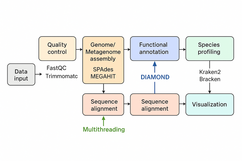
Microbial bioinformatics uses computational tools to analyze genomes, track evolution, and study functions in microorganisms, including bacteria and viruses.
Below is a sorted, step‑by‑step protocol integrating all commands and materials from your notes — organized into logical analysis phases. It outlines how to process whole‑genome data, annotate with Prokka, perform pan‑genome and SNP‑based phylogenetic analysis, and conduct resistome profiling and visualization.
Use WGS data to determine phylogenetic relationships based on MLST. Confirm species identity of isolates: E. coli, K. pneumoniae, A. baumannii complex, P. aeruginosa.
Example log output:
[10:19:59] Excluding ecoli.icdA.262 due to --exclude option
[10:19:59] If you like MLST, you're going to absolutely love cgMLST!
[10:19:59] Done.
Observation: No strain was close enough to be a suspected clonal strain (to be confirmed later with SNP‑based analysis).
3. Genome Annotation with Prokka
Cluster isolates into four species folders and annotate each genome separately.
5 (Optional). For A. baumannii with zero hits, run DIAMOND BLASTp against VFDB proteins.
#If you want to be extra thorough for A. baumannii. Because your VFDB nucleotide set returned zero for A. baumannii, you can cross-check with VFDB protein via DIAMOND:

# Build a DIAMOND db (once)
diamond makedb -in VFDB_proteins.faa -d vfdb_prot

# Query predicted proteins (Prokka .faa) per isolate
for F in fasta_abaumannii_cluster/*.fasta; do
  ISO=$(basename "$F" .fasta)
  prokka --cpus 8 --outdir prokka/$ISO --prefix $ISO "$F"
  diamond blastp -q prokka/$ISO/$ISO.faa -d vfdb_prot \
    -o abricate_vfdb/$ISO.vfdb_prot.tsv \
    -f 6 qseqid sseqid pident length evalue bitscore qcovhsp \
    --id 90 --query-cover 80 --max-target-seqs 1 --threads 8
done
8. Visualization with ggtree and Heatmaps
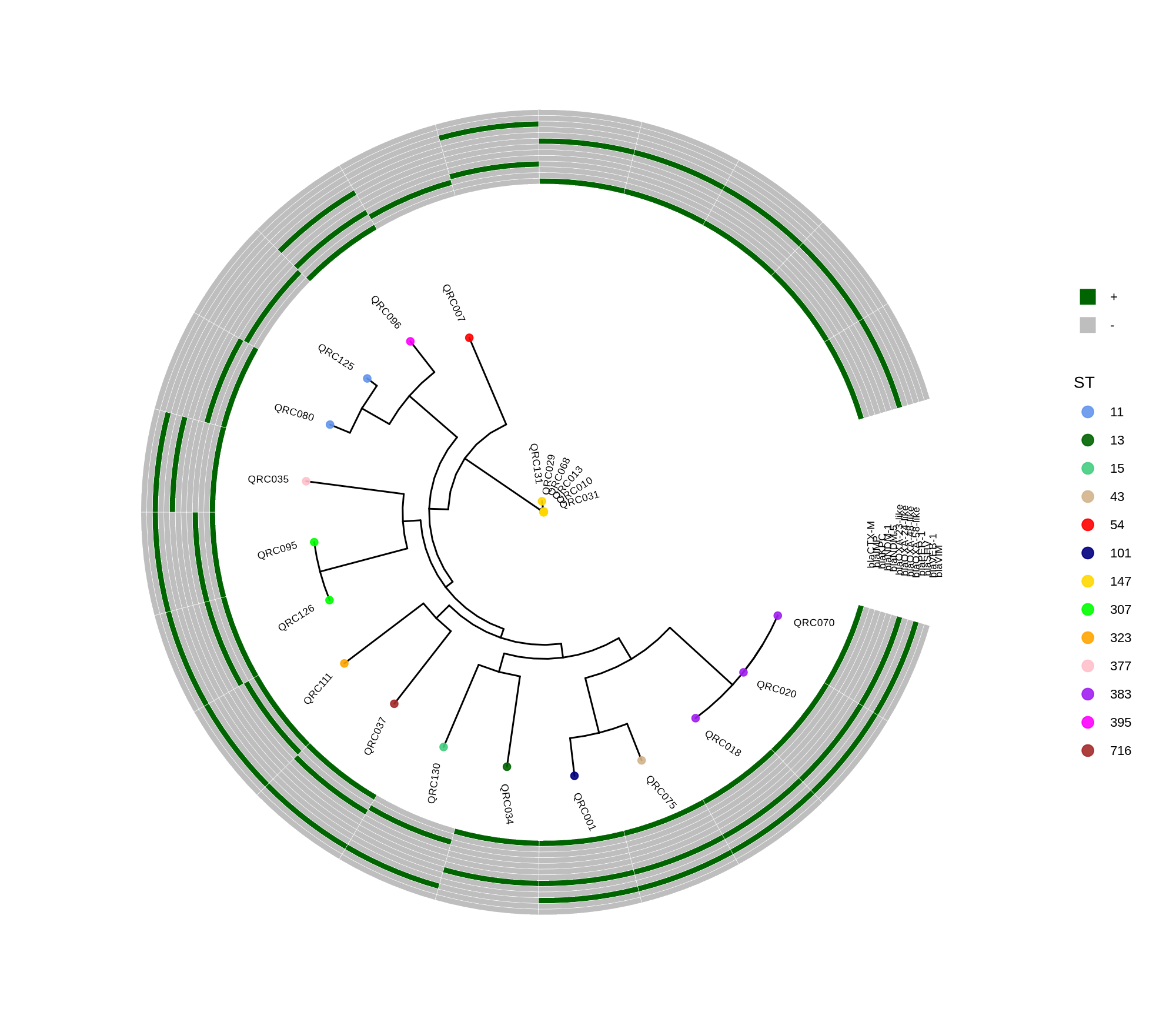
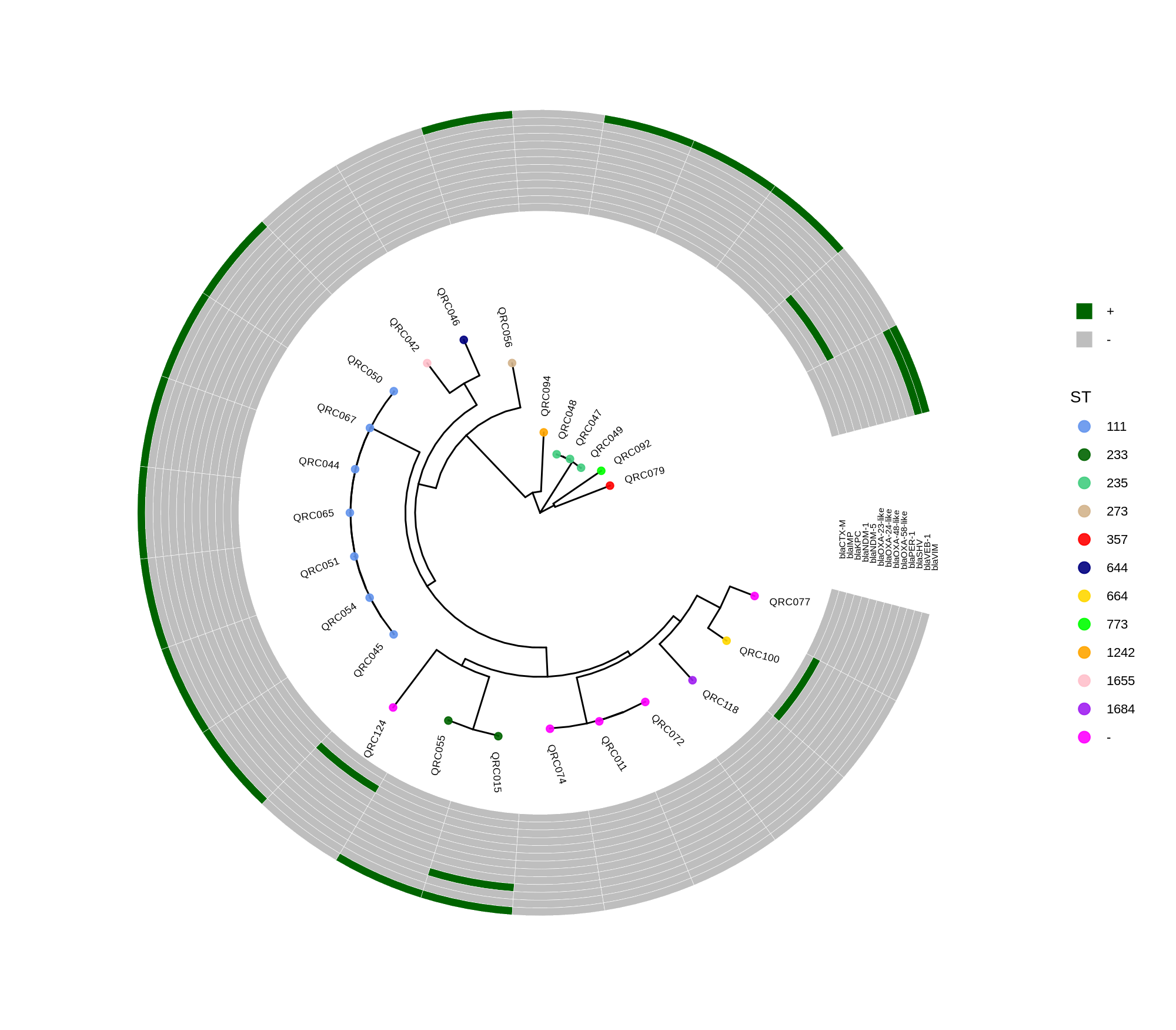
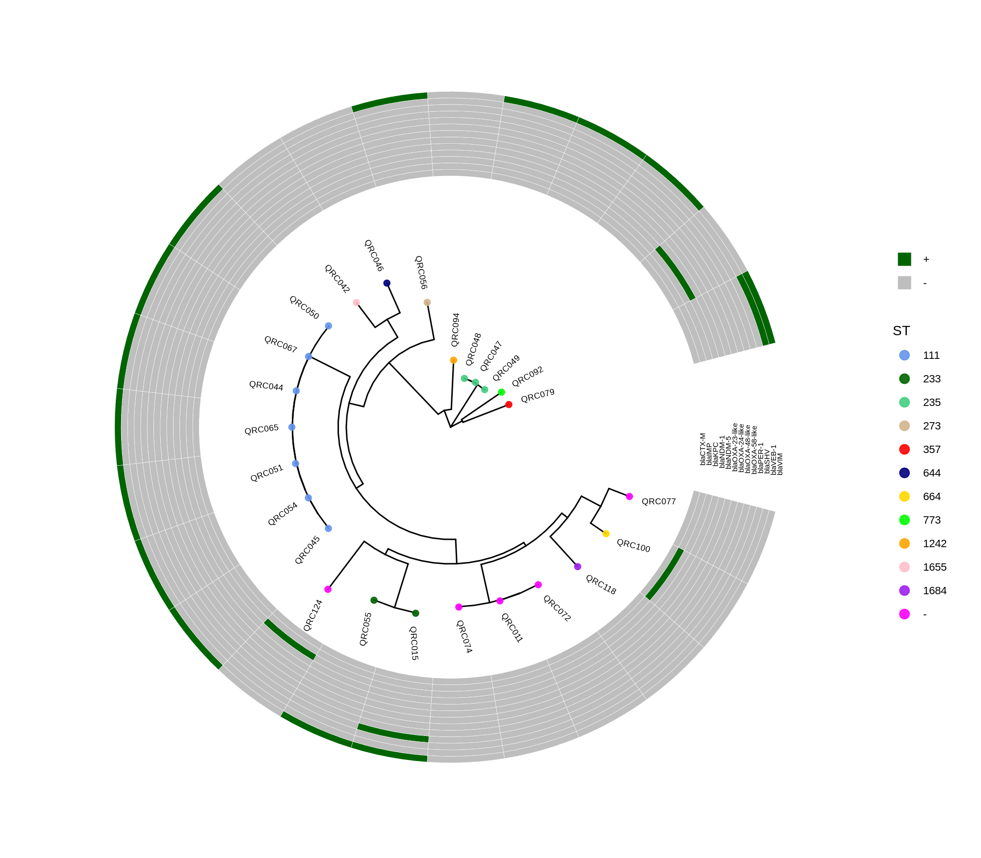
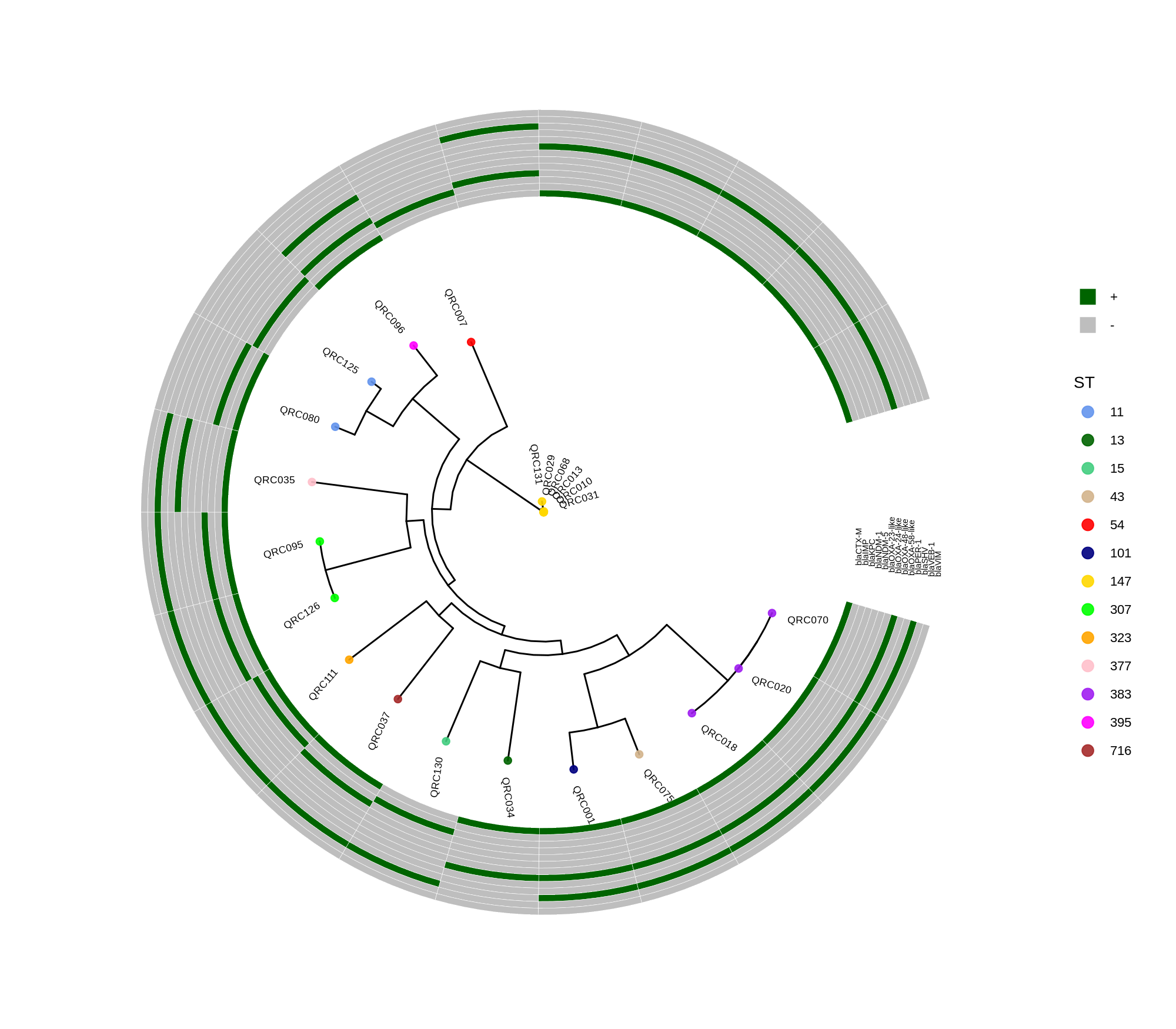
Render circular core genome trees and overlay selected ARGs or gene presence/absence matrices.
Key R snippet:
library(ggtree)
library(ggplot2)
library(dplyr)
info <- read.csv("typing_until_ecpA.csv", sep="\t")
tree <- read.tree("raxml-ng/snippy.core.aln.raxml.tree")
p <- ggtree(tree, layout='circular', branch.length='none') %<+% info +
     geom_tippoint(aes(color=ST), size=4) + geom_tiplab2(aes(label=name), offset=1)
gheatmap(p, heatmapData2, width=4, colnames_angle=45, offset=4.2)
Output: multi‑layer circular tree (e.g., ggtree_and_gheatmap_selected_genes.png).
9. Final Analyses and Reporting
Compute pairwise SNP distances and identify potential clonal clusters using species‑specific thresholds (e.g., ≤17 SNPs for E. coli).
If clones exist, retain one representative per cluster for subsequent Boruta analysis or CA/EA metrics.
Integrate ARG heatmaps to the trees for intuitive visualization of resistance determinants relative to phylogeny.
Protocol Description Summary
This workflow systematically processes WGS data from multiple bacterial species:
SNP‑distance computation (snp‑sites, snp‑dists) allows clonal determination and diversity quantification.
Resistome analysis (Abricate, Diamond) characterizes antimicrobial resistance and virulence determinants.
Visualization (ggtree + gheatmap) integrates tree topology with gene presence–absence or ARG annotations.
Properly documented, this end‑to‑end pipeline can serve as the Methods section for publication or as an online reproducible workflow guide.
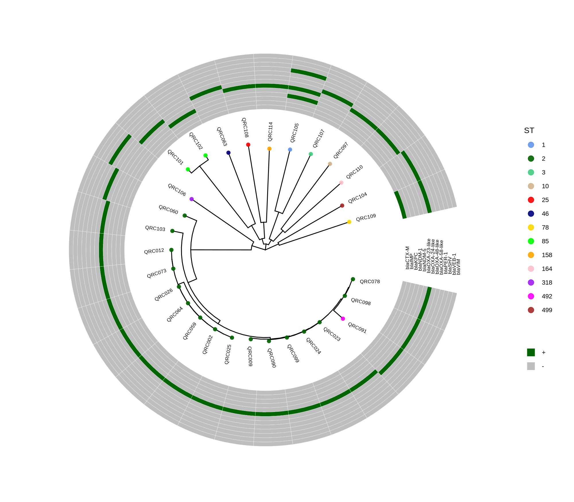
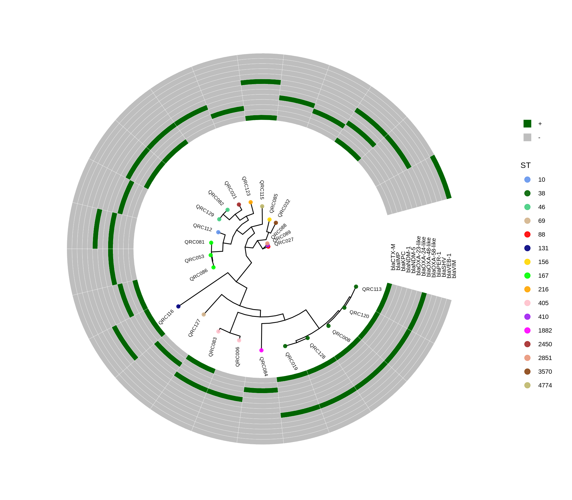
Methods (for the manuscript). Genomes were annotated with PROKKA v1.14.5 [1]. A pangenome was built with Roary v3.13.0 [2] using default settings (95% protein identity) to derive a gene presence/absence matrix. Core genes—defined as present in 99–100% of isolates by Roary—were individually aligned with MAFFT v7 [3] and concatenated; the resulting multiple alignment was used to infer a maximum-likelihood phylogeny in RAxML-NG [4] under GTR+G, with 1,000 bootstrap replicates [5] and a random starting tree. Trees were visualized with the R package ggtree [6] in circular layout; tip colors denote sequence type (ST), with MLST assigned via PubMLST/BIGSdb [7]; concentric heatmap rings indicate the presence (+) or absence (-) of resistance genes.
Seemann T. 2014. Prokka: rapid prokaryotic genome annotation. Bioinformatics 30:2068–2069.
Page AJ, Cummins CA, Hunt M, Wong VK, Reuter S, Holden MTG, Fookes M, Falush D, Keane JA, Parkhill J. 2015. Roary: rapid large-scale prokaryote pan genome analysis. Bioinformatics 31:3691–3693.
Katoh K, Standley DM. 2013. MAFFT multiple sequence alignment software version 7: improvements in performance and usability. Molecular Biology and Evolution 30:772–780.
Kozlov AM, Darriba D, Flouri T, Morel B, Stamatakis A, Wren J. 2019. RAxML-NG: a fast, scalable and user-friendly tool for maximum likelihood phylogenetic inference. Bioinformatics 35:4453–4455.
Felsenstein J. 1985. Confidence limits on phylogenies: an approach using the bootstrap. Evolution 39:783–791.
Yu G, Smith DK, Zhu H, Guan Y, Lam TT-Y. 2017. ggtree: an R package for visualization and annotation of phylogenetic trees. Methods in Ecology and Evolution 8(1):28–36.
Jolley KA, Bray JE, Maiden MCJ. 2018. Open-access bacterial population genomics: BIGSdb software, the PubMLST.org website and their applications. Wellcome Open Res 3:124.
This R script visualizes a phylogenetic tree of E. coli isolates using the ggtree and ggplot2 packages, annotated with sequence type (ST) colors and a heatmap showing the presence or absence of antimicrobial resistance genes. It creates several versions of the circular tree figure to adjust scaling and readability.
Key Steps
Load libraries and data
The code imports ggtree, ggplot2, and dplyr, reads isolate metadata (isolate_ecoli_.csv), and loads a phylogenetic tree file (ecoli_core_gene_tree_1000.raxml.bestTree).1112
Prepare metadata
It defines each isolate’s name and converts the sequence type (ST) into a categorical factor. A subset of columns (various bla resistance gene markers) is selected to create a heatmap data matrix, where each gene’s presence (“+”) or absence (“–”) will be visualized.
Define color schemes
Different STs are assigned distinct colors, and binary gene presence/absence states (“+”, “–”) mapped to “darkgreen” and “grey,” respectively.13
Plot tree with annotation
The main tree is plotted circularly using:
p <- ggtree(tree, layout='circular', branch.length='none') %<+% info +
     geom_tippoint(aes(color=ST)) + scale_color_manual(values=cols)
Tip labels are added for isolates, and STs are colored as per the legend.
Add heatmap (gene presence/absence)
The gheatmap() function appends the gene matrix to the tree, aligning rows with the tree tips and providing a heatmap of resistance gene patterns.1213
Export figures
Multiple PNGs are generated:
ggtree.png: Basic circular tree
ggtree_and_gheatmap_mibi_selected_genes.png: Tree + resistance gene heatmap
Scaled versions with adjusted offsets and spacing for improved readability and “true-scale” representations
Final Output
The resulting figures show a circular phylogenetic tree annotated by ST colors, accompanied by a ring-style heatmap indicating the distribution of key resistance genes across isolates. The layout adjustments (tree shrinking, offset tuning, width scaling) ensure legibility when genes or isolates are numerous.12131415161718192021222324252627282930
Match IDs: convert UniProt protein IDs to gene symbols to allow direct comparison with RNA-seq.
Merge datasets by gene_symbol and retain: protein_log2FC, protein_padj, rna_log2FC, rna_padj.
Classify each gene/protein into:
both_significant_same_direction
both_significant_opposite_direction
protein_only_significant
rna_only_significant
Subset analysis: examine proteins significant in proteomics but not in RNA-seq (and vice versa) to identify post-transcriptional regulation, stability, secretion/export, or translational effects.
If “Present via UniProt stream now” is 0, it usually indicates a streaming query/parse/limit issue; cached per‑accession FASTAs are valid and sufficient for alignment.
7) Why counts differ (e.g., 1173(1319) vs 1107; TSB 663 vs 650)
The aligner uses “unique, usable” FASTA sequences; duplicates, deprecated/secondary or invalid accessions, and empty/invalid sequences are filtered, so usable proteins can be fewer than attempted fetches.
TSB 663 vs 650: about 13 entries typically drop due to duplicate/merged IDs, obsolete accessions, decoy/contaminant-like strings, or missing gene symbols that prevent a 1‑to‑1 map with RNA-seq.
As mentioned, the IDs between proteomics and RNA‑seq were matched based on direct sequence alignment (ORF nucleotide sequences translated and aligned to UniProt protein FASTA) to ensure 1‑to‑1 mapping and unambiguous ID correspondence.
Please note that the recorded counts are constrained by the proteomics differentially expressed (DE) tables: for MH medium, 1107 proteins/genes; for TSB medium, 650. The RNA‑seq DE lists are larger overall, but the integration and comparisons are based on entities present in both proteomics and RNA‑seq.
For the overlap between the two datasets, each gene/protein was placed into one of five categories:
not_significant_in_either
rna_only_significant
protein_only_significant
both_significant_same_direction
both_significant_opposite_direction
The attached Excel file contains per‑comparison merged tables (protein_log2FC, protein_padj, rna_log2FC, rna_padj), category calls for each entry, and summary counts for quick review.
9) Notes \& assumptions
MH comparison blocks are read in 18h, 4h, 1h order from Ord_609 (three repeated “Log2 difference / q-value (Benjamini FDR)” blocks after intensities). If the template differs, adjust the mapping.
TSB comparisons are explicitly labeled (sbp vs Control at 1h/4h/18h) and are used verbatim.
Gene symbol preference: use proteomics-provided symbols (MH via GN=; TSB via Gene Symbol); otherwise fall back to RNA Preferred_name by locus to unify merge keys.
Significance: default padj < 0.05 for both datasets (set via –alpha). Add effect-size filters if needed.
10) TODOs
Cluster by presence across platforms: using TSB 650 and MH 1319 proteins, derive 5+1 groups; the +1 group contains genes not occurring in the proteomics results; Namely, RNA-only-present category: implemented—prefer set-difference on gene_symbol (RNA DE minus proteomics DE) per comparison to produce concise lists and avoid many‑to‑many expansions.
Re-run proteomics DE with Gunnar’s project scripts to expand DE coverage if needed.
 (plot-numpy1) python 1_filter_track.py

 #NOT necessary by reprocessing: (plot-numpy1) ./lake_files/2_generate_orig_lake_files.py

 (plot-numpy1) python 3_update_lake.py

 #PREPARE DIR position_2s_lakes by: mv updated_lakes/*_position_2s.lake position_2s_lakes
 #DEFINE input_dir = 'position_2s_lakes' and output_filename = 'position_2s.lake' in 4_merge_lake_files.py
 (plot-numpy1) python 4_merge_lake_files.py

 #Found 35 .lake files to merge. Merging...
 #✅ Merging complete!
 #   - Total unique H5 files: 35
 #   - Total kymograph entries: 35
 #   - Merged file saved as: 'position_2s.lake'

 #Found 37 .lake files to merge. Merging...
 #✅ Merging complete!
 #   - Total unique H5 files: 37
 #   - Total kymograph entries: 37
 #   - Merged file saved as: 'lifetime_5s_only.lake'
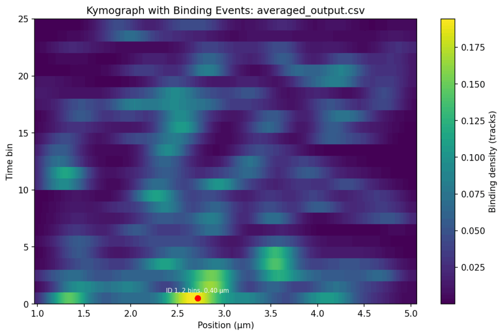
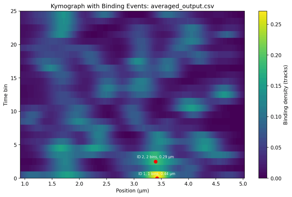
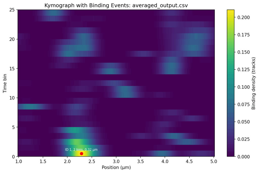
Overlap the track signals
{.alignnone}
{.alignnone}
{.alignnone}
# Change several filename to adapt the conventions
cd Binding_positions_60_timebins
mv p968_250702_502_10pN_ch4_0bar_b5_2_binding_position_blue.csv p968_250702_p502_10pN_ch4_0bar_b5_2_binding_position_blue.csv
mv p968_250702_502_10pN_ch4_0bar_b5_1_binding_position_blue.csv p968_250702_p502_10pN_ch4_0bar_b5_1_binding_position_blue.csv
mv p968_250702_502_10pN_ch4_0bar_b4_4_binding_position_blue.csv p968_250702_p502_10pN_ch4_0bar_b4_4_binding_position_blue.csv
mv p968_250702_502_10pN_ch4_0bar_b4_3_binding_position_blue.csv p968_250702_p502_10pN_ch4_0bar_b4_3_binding_position_blue.csv
mv p968_250702_502_10pN_ch4_0bar_b4_2_binding_position_blue.csv p968_250702_p502_10pN_ch4_0bar_b4_2_binding_position_blue.csv
mv p968_250702_502_10pN_ch4_0bar_b4_1_binding_position_blue.csv p968_250702_p502_10pN_ch4_0bar_b4_1_binding_position_blue.csv
mv p968_250702_502_10pN_ch4_0bar_b3_1_binding_position_blue.csv p968_250702_p502_10pN_ch4_0bar_b3_1_binding_position_blue.csv
mv p968_250702_502_10pN_ch4_0bar_b2_2_binding_position_blue.csv p968_250702_p502_10pN_ch4_0bar_b2_2_binding_position_blue.csv
mv p968_250702_502_10pN_ch4_0bar_b2_1_binding_position_blue.csv p968_250702_p502_10pN_ch4_0bar_b2_1_binding_position_blue.csv
mv p968_250702_502_10pN_ch4_0bar_b1_3_binding_position_blue.csv p968_250702_p502_10pN_ch4_0bar_b1_3_binding_position_blue.csv
mv p968_250702_502_10pN_ch4_0bar_b1_2_binding_position_blue.csv p968_250702_p502_10pN_ch4_0bar_b1_2_binding_position_blue.csv
mv p968_250702_502_10pN_ch4_0bar_b1_1_binding_position_blue.csv p968_250702_p502_10pN_ch4_0bar_b1_1_binding_position_blue.csv
# Sort the Binding_positions_60_timebins files into three direcories
mkdir ../tracks_p968_250702_p502/ ../tracks_p853_250706_p511/ ../tracks_p853_250706_p502/
mv p968_250702_p502*.csv ../tracks_p968_250702_p502/
mv p853_250706_p511*.csv ../tracks_p853_250706_p511/
mv p853_250706_p502*.csv ../tracks_p853_250706_p502/
cd ..; rmdir Binding_positions_60_timebins
# #p853_250706_p511
# event_id;start_bin;end_bin;avg_position;peak_size
# 1;57;57;1.706;0.143
# 2;40;42;2.019;0.142
# 3;44;45;2.014;0.134
# 4;0;6;2.146;0.143
# 5;25;25;3.208;0.143
# 6;27;27;3.181;0.124
# 7;42;42;3.559;0.143
# *8;0;0;3.929;0.143
# 9;34;38;4.135;0.143
# 10;42;44;4.591;0.148
# 11;47;50;4.667;0.144
# -->
# event_id;start_bin;end_bin;duration_bins;pos_range;avg_position;peak_size
# 1;56;56;1;0.256;1.706;0.143
# 2;39;41;3;0.256;2.019;0.142
# 3;43;44;2;0.229;2.014;0.134
# 4;0;5;6;0.243;2.152;0.138
# 5;24;24;1;0.269;3.208;0.143
# 6;26;26;1;0.216;3.181;0.124
# 7;41;41;1;0.269;3.559;0.143
# 8;33;37;5;0.256;4.135;0.143
# 9;41;43;3;0.377;4.591;0.148
# 10;46;49;4;0.404;4.667;0.144
#> (plot-numpy1) jhuang@WS-2290C:~/DATA/Data_Vero_Kymographs/Binding_positions$ python overlap_v16_calculate_average_matix.py
#1. Averaging: Compute the averaged and summed values at each (position, time_bin) point for tracks_p***_2507**_p***.
# ---- Filtering the first time bin 0 for all three groups tracks_p***_2507**_p*** ----
#rm tracks_p853_250706_p511/*_blue_filtered.csv
for f in ./tracks_p853_250706_p511/*.csv; do
python -c "import pandas as pd; \
df=pd.read_csv('$f', sep=';'); \
df.drop(columns=['time bin 0']).to_csv('${f%.csv}_filtered.csv', sep=';', index=False)"
done
rm tracks_p853_250706_p511/*_binding_position_blue.csv
for f in ./tracks_p853_250706_p502/*.csv; do
python -c "import pandas as pd; \
df=pd.read_csv('$f', sep=';'); \
df.drop(columns=['time bin 0']).to_csv('${f%.csv}_filtered.csv', sep=';', index=False)"
done
rm tracks_p853_250706_p502/*_binding_position_blue.csv
for f in ./tracks_p968_250702_p502/*.csv; do
python -c "import pandas as pd; \
df=pd.read_csv('$f', sep=';'); \
df.drop(columns=['time bin 0']).to_csv('${f%.csv}_filtered.csv', sep=';', index=False)"
done
rm tracks_p968_250702_p502/*_binding_position_blue.csv
#hard-coding the path: file_list = glob.glob("tracks_p853_250706_p502/*_binding_position_blue_filtered.csv")
python 1_combine_kymographs.py
mkdir tracks_p853_250706_p502_averaged
mv tracks_p853_250706_p502/averaged_output.csv tracks_p853_250706_p502_averaged
#hard-coding the path: file_list = glob.glob("tracks_p853_250706_p502_averaged/averaged_output.csv")
python 1_combine_kymographs.py
mkdir tracks_p853_250706_p502_sum
mv tracks_p853_250706_p502/sum_output.csv tracks_p853_250706_p502_sum
#hard-coding the path: file_list = glob.glob("tracks_p853_250706_p502_sum/sum_output.csv")
python 1_combine_kymographs.py
python 2_summarize_binding_events.py tracks_p853_250706_p502_binding_events
mv summaries tracks_p853_250706_p502_binding_event_summaries
# -------------------- The following steps are deprecated --------------------
#After adapting the dir PARAMETERS 'tracks_p853_250706_p511' in the following two python-scripts
python overlap_v16_calculate_average_matix.py
python overlap_v17_draw_plot.py
cd tracks_p853_250706_p511/debug_outputs/
cut -d';' -f1-4 averaged_output_events.csv >f1_4
cut -d';' -f6-7 averaged_output_events.csv >f6_7
paste -d';' f1_4 f6_7 > tracks_p853_250706_p511.csv
mv averaged_output_events.png tracks_p853_250706_p511.png
#After adapting the dir parameter 'tracks_p853_250706_p502' in the following two python-scripts
python overlap_v16_calculate_average_matix.py
python overlap_v17_draw_plot.py
cd tracks_p853_250706_p502/debug_outputs/
cut -d';' -f1-4 averaged_output_events.csv >f1_4
cut -d';' -f6-7 averaged_output_events.csv >f6_7
paste -d';' f1_4 f6_7 > tracks_p853_250706_p502.csv
mv averaged_output_events.png tracks_p853_250706_p502.png
#After adapting the dir parameter 'tracks_p968_250702_p502' in the following two python-scripts
python overlap_v16_calculate_average_matix.py
python overlap_v17_draw_plot.py
cd tracks_p968_250702_p502/debug_outputs/
cut -d';' -f1-4 averaged_output_events.csv >f1_4
cut -d';' -f6-7 averaged_output_events.csv >f6_7
paste -d';' f1_4 f6_7 > tracks_p968_250702_p502.csv
mv averaged_output_events.png tracks_p968_250702_p502.png
~/Tools/csv2xls-0.4/csv_to_xls.py \
tracks_p853_250706_p511/debug_outputs/tracks_p853_250706_p511.csv \
tracks_p853_250706_p502/debug_outputs/tracks_p853_250706_p502.csv \
tracks_p968_250702_p502/debug_outputs/tracks_p968_250702_p502.csv \
-d$';' -o binding_events.xls;
#Correct the sheet names in binding_events.xls.
# --> The FINAL results are binding_events.xls and tracks_p***_25070*_p5**/debug_outputs/tracks_p***_25070*_p5**.png.
# ------ END ------
#2. Threshold-based detection: Apply a signal threshold (e.g., 0.16) to identify bound states at each position and time bin.
#3. Merging neighboring events: Combine adjacent bound regions in both position and time.
#4. Event filtering: Only merged events that satisfy the following conditions are reported as binding events and annotated in the plot:
* min_duration = 1 # minimum number of time bins
* min_range = 0.08 μm # minimum position spread for an event
5. Event statistics: Calculate time bin ranges, durations, peak sizes, and average positions for each event.
NEW_ADAPT: I have checked the files again, and those marked with 'my_...' are filtered by position and time. I sent you the unfiltered files so that you could create the nice heat maps that you made. So everything is correct. Could you do me two more favours?
Firstly, would it be possible to send me the heat maps of the '..._averaged_output_events' without the red dot, ID, bins and position?
Secondly, would it be possible to have a similar binding intensity scale for all three samples?
#--> Done with the new python code. TODO: update the post in bioinformatics.cc.
Thirdly, could you create the same heat maps, but with only the tracks above 5 seconds? That would be great.
#Solution for 3rd point: delete the input files the second columns for "ignoring the first time bin (namely time bin 0). "
#Additionally: delete the column "duration_bins" in averaged_output_events.csv and convert csv to Excel-file using csv2xls; TODO: observe in the new output Excel-files, the start_bin and end_bin, the numbers will be changed?
“Why do my alpha diversity values differ between groups?”
“Why is mpse_abund$Group full of `
` values?”
💡 For debugging R code (e.g., MicrobiotaProcess, phyloseq, S4 objects) → Use Qwen3-Coder.
For broader scientific reasoning alongside code → consider Qwen3-Max after fixing the code with Qwen3-Coder.