Protected: Table X. Logical summary of the biochemical and phenotypic consequences of efflux pump deletions under chloramphenicol in A. baumannii ATCC19606.”
Enter your password to view comments.
| 方面 | PNAS 2018:海马、空间学习与“关键期” | J Neurosci 2019:前额叶、精神分裂症相关表型 |
|---|---|---|
| 研究脑区 | 海马 (Hippocampus) | 前额叶皮层 (PFC) |
| 核心问题 | 海马空间学习是否存在依赖 Arc 的发育关键期? | Arc 缺失是否会导致精神分裂症样行为和 PFC 功能异常? |
| 主要方法 | – 不同时间窗 Arc KO 小鼠 (常规/早期 P7+/晚期 P21+) – Morris 水迷宫、情境恐惧记忆 – 海马 LFP (theta, gamma, ripple) |
– 同样 KO 小鼠 – PFC LFP (theta, gamma) + 切片电生理 (E/I 平衡、网络增益) – 社交、工作记忆 (Y 迷宫)、PPI、开放场、安非他命反应、癫痫易感性等 |
| 主要结论 | – Arc 在出生后首月海马高表达,形成发育关键期 – 早期敲除永久损害网络振荡及成年空间学习 – 晚期敲除不影响学习但仍需 Arc 存储长期记忆 一句话:Arc 决定海马空间学习网络的“发育窗口” |
– 早期/全身 KO 削弱 PFC 振荡及突触功能 (网络“长歪”) – 但无典型精神分裂症行为缺陷 (社交、工作记忆、PPI、多巴胺正常) – Arc 删除扰乱 PFC 网络但不足以产生精神分裂症样行为 一句话:Arc 缺失单独不足以造成精神分裂症 |
| 结论导向 | Arc 的必要性 + 关键期:特定发育阶段对海马网络成熟关键 | Arc 删除为不充分条件:需 Arc 失调 + 其他因素组合 |
| 方法侧重 | 行为 + 海马 LFP (theta/gamma/ripple) | PFC LFP + 切片电生理 + 全面精神分裂症行为/多巴胺/癫痫测试 |
针对第 9、10、11 组以及混合的 pre-FMT 组的 PCA 和多样性分析
筛选条件:Group 9(J1–4, J10, J11)、Group 10(K1–K6)、Group 11(L2–L6)以及 pre-FMT(G1–G6, H1–H6, I1–I6)
1.1 这些组之间在 α 多样性或 β 多样性方面是否存在显著差异?你能否为此生成一个 PCoA 图?
1.2 在仅比较第 9、10 和 11 组时,α 多样性或 β 多样性之间是否存在显著差异?你能否也为此生成一个 PCoA 图?
1.3 第 9 组与第 10 组之间有哪些差异表达的基因(DEGs)?
1.4 第 9 组与第 10 组之间是否存在差异富集/差异表达的通路?
1.5 你是否可以使用 R 绘制一棵系统聚类树(树状图),包含数据集中检测到的所有细菌科(bacterial families)?我附了一篇论文作为示例(Figure 1C)。
Group 3 与 Group 4 之间的通路分析
筛选条件:Group 3:C1–C7;Group 4:E1–E10。
是否可以请你对 Group 3 vs Group 4 做一次通路分析?
2022 年数据集(第一组筛选条件)
筛选条件:Group 1:1, 2, 7, 6;Group 5:29, 30, 31。
这些组之间在 α 多样性或 β 多样性方面是否存在显著差异?你能否为此生成一个 PCoA 图?
有哪些 DEGs?
是否存在差异富集/差异表达的通路?
2022 年数据集(第二组筛选条件)
筛选条件:Group 1:1, 2, 7, 6;Group 5:29, 30, 31;Group 2(不加筛选);Group 6(不加筛选)。
这些组之间在 α 多样性或 β 多样性方面是否存在显著差异?你能否为此生成一个 PCoA 图?
微生物组分析的方法部分
我们已经写好了材料和方法部分,其中包含微生物组分析的内容,我已将这一部分附在邮件中。你有没有什么意见?特别是你认为是否还需要补充描述 QC(质控)分析的内容?
Microbiome analysis(微生物组分析)
在所示时间点,于上午 9–10 点之间采集小鼠粪便样本,并立即在 -80°C 冻存直至使用。DNA 提取使用 QIAamp Fast DNA Stool Mini Kit(Qiagen, #51604),并根据已发表的小鼠粪便专用方案进行操作⁸。简而言之,粪便颗粒在 Precellys® 24 匀浆器(Bertin Technologies)中、使用 Soil grinding tubes(Bertin Technologies, #SK38)进行均质处理,随后按照试剂盒说明书提取 DNA。通过 Nanodrop 测定 DNA 产量,并将浓度调至 10 ng/µl。16S rRNA 扩增子(V3–V4 区域)采用带有 Illumina 接头通用序列的简并引物进行扩增:前向引物 F(5′- TCGTCGGCAGCGTCAGATGTGTATAAGAGACAGCCTACGGGNGGCWGCAG-3′),反向引物 R(5′-GTCTCGTGGGCTCGGAGATGTGTATAAGAGACAGGACTACHVGGG-TATCTAATCC-3′),具体方法参考已发表的方案⁹,¹⁰。随后使用 Illumina Nextera XT Index Kit(Illumina, #FC-131-1001)对样本进行多重上样,构建带条形码的文库。文库在 MiSeq 平台(Illumina, #MS-102-2003)上进行 500PE 测序。
QC
不同组之间微生物群落组成的差异使用 PERMANOVA(置换多元方差分析)进行评估,基于 R 包 vegan 中的 adonis 函数,设置 9999 次置换。该分析基于 Bray–Curtis 距离矩阵,该矩阵综合考虑了物种的有无以及各物种在每个样本中的相对丰度。该方法用于评估不同组之间整体群落组成是否存在显著差异。
群体间的差异丰度分析使用 R 包 DESeq2 完成,该方法通过负二项式广义线性模型对计数数据进行建模¹¹。在气泡图中,x 轴表示相对丰度的 log₂ 倍数变化,每个气泡代表一个 OTU,气泡颜色表示其所属的细菌目(bacterial order),气泡大小表示经过 Benjamini–Hochberg 校正后的调整 p 值。
关于 PCoA 和 PCA 的问题
我们目前还不是完全确定你所做的分析是主坐标分析(PCoA)还是主成分分析(PCA)。你能否就此再给一些说明或评论?
第 9、10、11 组及混合 pre-FMT 组的 PCA 和多样性分析
你之前已经向我们展示过,这些组在 α 多样性和 β 多样性方面存在显著差异。我们能否据此得出结论:每一组在 α 和 β 多样性上都与所有其他组显著不同?如果不能,是否可以做一个事后检验(例如 Bonferroni 校正的 post-hoc 分析),来查看哪些组在 α 或 β 多样性上存在显著差异?在这里,我们主要感兴趣的比较是:9 vs 10,9 vs 11,10 vs 11。
通路分析:第 9 组 vs 第 10 组
是否可以预先筛选我们感兴趣的通路?在这里,我们特别想关注参与短链脂肪酸(SCFAs)生成的相关通路。这个在分析上可行吗?你对这样的做法有什么看法或建议?
2022 年数据集:第 1、2、5 和 6 组
在第 1 组和第 5 组之间,是否能检测到任何差异表达基因(DEGs)?
你之前已经向我们展示过,第 1、2、5 和 6 组之间在 β 多样性上存在显著差异。结合我在第一个问题中的疑问:这些组在 β 多样性上是否彼此之间都显著不同,还是说我们需要进行事后分析(post-hoc)来判断具体是哪些组之间存在显著差异?在这里,我们主要关心的比较是 1 vs 5 和 2 vs 6。你能帮我们一起解读这些结果吗?
The table lists Hamburg state schools’ 2025 Abitur average grades and graduate counts, now with an index column as first column.1
| # | School (English [German]) | Avg. grade | Number of graduates |
|---|---|---|---|
| 1 | Oberalster Grammar School [Gymnasium Oberalster] | 1.83 | 86 |
| 2 | Johanneum Academic School [Gelehrtenschule des Johanneums] | 1.91 | 104 |
| 3 | Christianeum [Christianeum] | 1.93 | 108 |
| 4 | Second Educational Path Campus (former Hansa-Kolleg) [Campus Zweiter Bildungsweg (eh. Hansa-Kolleg)] | 1.94 | 14 |
| 5 | Buckhorn Grammar School [Gymnasium Buckhorn] | 1.95 | 122 |
| 6 | Helene-Lange Grammar School [Helene-Lange-Gymnasium] | 1.96 | 123 |
| 7 | Altona Grammar School [Gymnasium Altona] | 2.00 | 109 |
| 8 | Albert Schweitzer Grammar School [Albert-Schweitzer-Gymnasium] | 2.05 | 109 |
| 9 | Othmarschen Grammar School [Gymnasium Othmarschen] | 2.05 | 88 |
| 10 | Walddörfer Grammar School [Walddörfer-Gymnasium] | 2.07 | 155 |
| 11 | Ohlstedt Grammar School [Gymnasium Ohlstedt] | 2.10 | 46 |
| 12 | Rissen Grammar School [Gymnasium Rissen] | 2.10 | 82 |
| 13 | Blankenese Grammar School [Gymnasium Blankenese] | 2.11 | 115 |
| 14 | Hochrad Grammar School [Gymnasium Hochrad] | 2.12 | 147 |
| 15 | Winterhude Community School [Stadtteilschule Winterhude] | 2.14 | 69 |
| 16 | Alstertal Grammar School [Gymnasium Alstertal] | 2.15 | 60 |
| 17 | Emilie-Wüstenfeld Grammar School [Emilie-Wüstenfeld-Gymnasium] | 2.16 | 121 |
| 18 | Friedrich-Ebert Grammar School [Friedrich-Ebert-Gymnasium] | 2.17 | 63 |
| 19 | Grootmoor Grammar School [Gymnasium Grootmoor] | 2.19 | 118 |
| 20 | Lerchenfeld Grammar School [Gymnasium Lerchenfeld] | 2.19 | 118 |
| 21 | Alter Teichweg Community School [Grund- und Stadtteilschule Alter Teichweg] | 2.20 | 125 |
| 22 | Hummelsbüttel Grammar School [Gymnasium Hummelsbüttel] | 2.20 | 74 |
| 23 | Eppendorf Grammar School [Gymnasium Eppendorf] | 2.21 | 91 |
| 24 | Kaiser-Friedrich-Ufer Grammar School [Gymnasium Kaiser-Friedrich-Ufer] | 2.21 | 95 |
| 25 | Marion Dönhoff Grammar School [Marion Dönhoff Gymnasium] | 2.21 | 75 |
| 26 | Matthias-Claudius Grammar School [Matthias-Claudius-Gymnasium] | 2.22 | 107 |
| 27 | Bergedorf Community School [Stadtteilschule Bergedorf] | 2.23 | 80 |
| 28 | Hansa Grammar School Bergedorf [Hansa-Gymnasium Bergedorf] | 2.24 | 104 |
| 29 | Bornbrook Grammar School [Gymnasium Bornbrook] | 2.25 | 72 |
| 30 | Ohmoor Grammar School [Gymnasium Ohmoor] | 2.25 | 156 |
| 31 | Wilhelm Grammar School [Wilhelm-Gymnasium] | 2.25 | 64 |
| 32 | Klosterschule Grammar School [Gymnasium Klosterschule] | 2.27 | 111 |
| 33 | Lohbrügge Grammar School [Gymnasium Lohbrügge] | 2.28 | 105 |
| 34 | Meiendorf Grammar School [Gymnasium Meiendorf] | 2.28 | 84 |
| 35 | Carl-von-Ossietzky Grammar School [Carl-von-Ossietzky-Gymnasium] | 2.29 | 92 |
| 36 | Max Brauer School [Max-Brauer-Schule] | 2.29 | 76 |
| 37 | Vocational School for Plant and Construction Engineering at Inselpark [Berufliche Schule Anlagen- und Konstruktionstechnik am Inselpark] | 2.32 | 13 |
| 38 | Rahlstedt Grammar School [Gymnasium Rahlstedt] | 2.32 | 110 |
| 39 | Allee Grammar School [Gymnasium Allee] | 2.33 | 107 |
| 40 | Bondenwald Grammar School [Gymnasium Bondenwald] | 2.33 | 93 |
| 41 | Osterbek Grammar School [Gymnasium Osterbek] | 2.33 | 45 |
| 42 | Alexander-von-Humboldt Grammar School [Alexander-von-Humboldt-Gymnasium] | 2.34 | 67 |
| 43 | Vocational School Am Lämmermarkt [Berufliche Schule Am Lämmermarkt] | 2.34 | 40 |
| 44 | Heidberg Grammar School [Gymnasium Heidberg] | 2.35 | 77 |
| 45 | Albrecht-Thaer Grammar School [Albrecht-Thaer-Gymnasium] | 2.37 | 92 |
| 46 | Vocational School for Banking, Insurance and Law with Vocational Grammar School St. Pauli [Berufliche Schule für Banken, Versicherungen und Recht mit Beruflichem Gymnasium St. Pauli] | 2.38 | 33 |
| 47 | Corveystraße Grammar School [Gymnasium Corveystraße] | 2.39 | 118 |
| 48 | Finkenwerder Grammar School [Gymnasium Finkenwerder] | 2.39 | 33 |
| 49 | Blankenese Community School [Stadtteilschule Blankenese] | 2.40 | 109 |
| 50 | Erich Kästner School [Erich Kästner Schule] | 2.41 | 57 |
| 51 | Farmsen Grammar School [Gymnasium Farmsen] | 2.41 | 62 |
| 52 | Walddörfer Community School [Stadtteilschule Walddörfer] | 2.41 | 61 |
| 53 | Allermöhe Grammar School [Gymnasium Allermöhe] | 2.42 | 61 |
| 54 | Oldenfelde Grammar School [Gymnasium Oldenfelde] | 2.42 | 73 |
| 55 | Julius-Leber School [Julius-Leber-Schule] | 2.42 | 112 |
| 56 | Dörpsweg Grammar School [Gymnasium Dörpsweg] | 2.43 | 80 |
| 57 | Margaretha-Rothe Grammar School [Margaretha-Rothe-Gymnasium] | 2.44 | 64 |
| 58 | Meiendorf Community School [Stadtteilschule Meiendorf] | 2.45 | 44 |
| 59 | Gyula Trebitsch School Tonndorf (G8) [Gyula Trebitsch Schule Tonndorf (G8)] | 2.45 | 24 |
| 60 | Struensee Grammar School [Struensee Gymnasium] | 2.47 | 74 |
| 61 | Goethe School Harburg [Goethe-Schule-Harburg] | 2.48 | 123 |
| 62 | Heinrich-Hertz School (G8) [Heinrich-Hertz-Schule (G8)] | 2.48 | 38 |
| 63 | Louise Weiss Grammar School [Louise Weiss Gymnasium] | 2.48 | 59 |
| 64 | Nelson Mandela School in Kirchdorf [Nelson-Mandela-Schule im Stadtteil Kirchdorf] | 2.49 | 59 |
| 65 | Kurt-Körber Grammar School [Kurt-Körber-Gymnasium] | 2.50 | 43 |
| 66 | Poppenbüttel Community School [Stadtteilschule Poppenbüttel] | 2.50 | 52 |
| 67 | Lise-Meitner Grammar School [Lise-Meitner-Gymnasium] | 2.53 | 83 |
| 68 | Altona Community School [Stadtteilschule Altona] | 2.54 | 38 |
| 69 | Bergedorf Community School (dual-qualifying track) [Stadtteilschule Bergedorf (doppelt qualifizierender Bildungsgang)] | 2.55 | 11 |
| 70 | City Nord Vocational School [Berufliche Schule City Nord] | 2.56 | 26 |
| 71 | Hamburg-Harburg Vocational School [Berufliche Schule Hamburg-Harburg] | 2.56 | 11 |
| 72 | Ida Ehre School [Ida Ehre Schule] | 2.57 | 86 |
| 73 | Goethe Grammar School [Goethe-Gymnasium] | 2.58 | 76 |
| 74 | Charlotte-Paulsen Grammar School [Charlotte-Paulsen-Gymnasium] | 2.59 | 62 |
| 75 | Fritz-Schumacher School [Fritz-Schumacher-Schule] | 2.59 | 46 |
| 76 | Am Heidberg Community School [Stadtteilschule Am Heidberg] | 2.59 | 60 |
| 77 | Vocational School for Social Pedagogy – Anna Warburg School [Berufliche Schule für Sozialpädagogik – Anna-Warburg-Schule] | 2.60 | 25 |
| 78 | Eppendorf Community School [Grund- und Stadtteilschule Eppendorf] | 2.60 | 55 |
| 79 | Helmut Schmidt Grammar School [Helmut-Schmidt-Gymnasium] | 2.60 | 83 |
| 80 | Am Hafen Community School [Stadtteilschule Am Hafen] | 2.60 | 66 |
| 81 | Fischbek-Falkenberg Community School [Stadtteilschule Fischbek-Falkenberg] | 2.60 | 42 |
| 82 | Second Educational Path Campus [Campus Zweiter Bildungsweg] | 2.61 | 58 |
| 83 | Marienthal Grammar School [Gymnasium Marienthal] | 2.63 | 67 |
| 84 | Lessing Community School [Lessing-Stadtteilschule] | 2.64 | 89 |
| 85 | Horn Community School [Stadtteilschule Horn] | 2.64 | 64 |
| 86 | Lohbrügge Community School [Stadtteilschule Lohbrügge] | 2.64 | 80 |
| 87 | Niendorf Community School [Stadtteilschule Niendorf] | 2.64 | 53 |
| 88 | Mümmelmannsberg Community School [Stadtteilschule Mümmelmannsberg] | 2.66 | 48 |
| 89 | Oldenfelde Community School [Stadtteilschule Oldenfelde] | 2.67 | 35 |
| 90 | Irena Sendler School [Irena-Sendler-Schule] | 2.68 | 89 |
| 91 | Hamburg-Mitte Community School [Stadtteilschule Hamburg-Mitte] | 2.68 | 45 |
| 92 | Max-Schmeling Community School [Max-Schmeling-Stadtteilschule] | 2.70 | 37 |
| 93 | Esther Bejarano School [Esther Bejarano Schule] | 2.70 | 52 |
| 94 | Flottbek Community School [Stadtteilschule Flottbek] | 2.70 | 13 |
| 95 | Wilhelmsburg Community School [Stadtteilschule Wilhelmsburg (OSW)] | 2.71 | 18 |
| 96 | Elisabeth-Lange School [Elisabeth-Lange-Schule] | 2.73 | 33 |
| 97 | Helmuth Hübener Community School [Stadtteilschule Helmuth Hübener] | 2.73 | 59 |
| 98 | Richard-Linde-Weg Community School [Stadtteilschule Richard-Linde-Weg] | 2.73 | 39 |
| 99 | Otto Hahn School [Otto-Hahn-Schule] | 2.77 | 62 |
| 100 | Stübenhofer Weg Community School (OSW) [Stadtteilschule Stübenhofer Weg (OSW)] | 2.77 | 11 |
| 101 | Heinrich-Hertz School (G9) [Heinrich-Hertz-Schule (G9)] | 2.76 | 74 |
| 102 | Emil Krause School [Emil Krause Schule] | 2.80 | 61 |
| 103 | Gyula Trebitsch School Tonndorf (G9) [Gyula Trebitsch Schule Tonndorf (G9)] | 2.80 | 67 |
| 104 | Geschwister-Scholl Community School [Geschwister-Scholl-Stadtteilschule] | 2.85 | 33 |
| 105 | Lurup Community School [Stadtteilschule Lurup] | 2.85 | 55 |
| 106 | Gretel Bergmann School [Gretel-Bergmann-Schule] | 2.90 | 35 |
| 107 | Bramfeld Community School [Stadtteilschule Bramfeld] | 2.92 | 25 |
| 108 | Finkenwerder Community School [Stadtteilschule Finkenwerder] | 2.97 | 16 |
| 109 | Öjendorf Community School [Stadtteilschule Öjendorf] | 2.96 | 13 |
| 110 | Altrahlstedt Community School [Grund- und Stadtteilschule Altrahlstedt] | 3.00 | 13 |
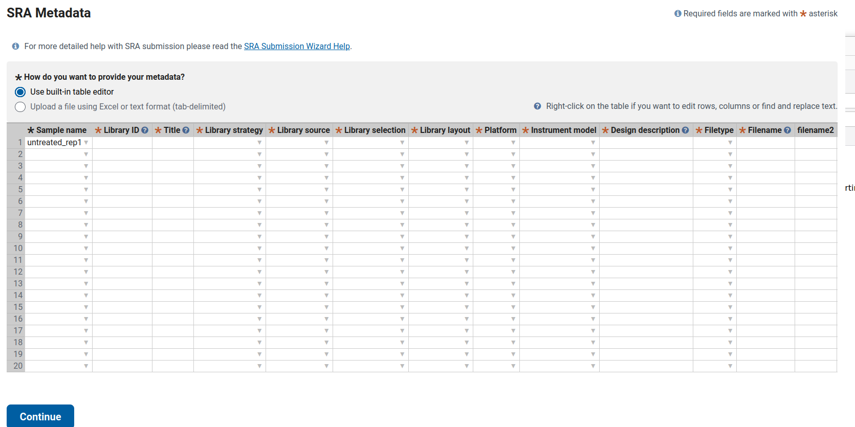
This guide explains how to complete the SRA metadata table for ten bulk RNA-seq samples derived from human skin organoids (SkOs). It includes one fully filled example row and shows the pattern to follow for the remaining samples.
According to the Methods section, all samples correspond to bulk RNA-seq using Lexogen RiboCop rRNA depletion and the Lexogen RNA-Seq V2 library kit. Sequencing was performed as single-end 1×83 bp reads on the Illumina NextSeq 500.
Therefore, the following columns remain identical for all samples (untreated_rep1 … HSV_d8_rep2):
untreated_rep1, HSV_d4_rep2, etc.).untreated_rep1 → LIB01
untreated_rep2 → LIB02
HSV_d2_rep1 → LIB03
…
HSV_d8_rep2 → LIB10Alternatively, a more descriptive format such as SkO_bulk_untreated_rep1 is acceptable. The key requirement is that all IDs are unique.
Examples:
untreated_rep1 → Bulk RNA-seq of human skin organoid (SkO), untreated, replicate 1
untreated_rep2 → Bulk RNA-seq of human skin organoid (SkO), untreated, replicate 2
HSV_d2_rep1   → Bulk RNA-seq of human skin organoid (SkO) infected with Human alphaherpesvirus 1 (HSV-1), 2 dpi, replicate 1
HSV_d4_rep2   → Bulk RNA-seq of human skin organoid (SkO) infected with Human alphaherpesvirus 1 (HSV-1), 4 dpi, replicate 2
Repeat this pattern for 6 dpi and 8 dpi samples.
Bulk RNA-seq of human hair-bearing skin organoids (SkOs) derived from hiPSC line UKEi001-A. Total RNA from two organoids per condition was pooled, depleted of rRNA (Lexogen RiboCop rRNA Depletion Kit for Human/Mouse/Rat V2), and libraries were prepared with the Lexogen RNA-Seq V2 Library Prep Kit with UDIs (short insert variant). Libraries were sequenced as 1×83 bp single-end reads on an Illumina NextSeq 500.
Then append the condition information as follows:
untreated_rep1 → untreated_rep1.fastq.gz
untreated_rep2 → untreated_rep2.fastq.gz
HSV_d2_rep1   → HSV_d2_rep1.fastq.gz
…
- **filename2:** leave blank (used only for paired-end libraries).| Column | Example Entry |
|---|---|
| Sample name | untreated_rep1 |
| Library ID | LIB01 |
| Title | Bulk RNA-seq of human skin organoid (SkO), untreated, replicate 1 |
| Library strategy | RNA-Seq |
| Library source | TRANSCRIPTOMIC |
| Library selection | RANDOM |
| Library layout | SINGLE |
| Platform | ILLUMINA |
| Instrument model | Illumina NextSeq 500 |
| Design description | Bulk RNA-seq of human hair-bearing skin organoids (SkOs) derived from hiPSC line UKEi001-A. Total RNA from two organoids per condition was pooled, depleted of rRNA (Lexogen RiboCop rRNA Depletion Kit for Human/Mouse/Rat V2) and libraries were prepared with the Lexogen RNA-Seq V2 Library Prep Kit with UDIs (short insert variant). Libraries were sequenced as 1×83 bp single-end reads on an Illumina NextSeq 500. Condition: untreated control. |
| Filetype | fastq |
| Filename | untreated_rep1.fastq.gz |
| filename2 | (blank) |
After completing this first row, copy and adjust the fields (Library ID, Title, Design description condition, and Filename) for the other nine samples accordingly.
Varicella-Zoster Virus (VZV) in complex skin organoids is about using advanced 3D human skin models to understand how VZV infects, spreads, and interacts with host immunity in its most relevant organ: the skin. 这些类器官尽量重建了人皮肤的层次结构和细胞多样性,使得对VZV的研究比传统二维细胞培养更接近真实感染情境。2345
VZV 的致病性高度依赖其在表皮角质形成细胞中的复制,这最终形成充满高滴度游离病毒的水疱,是人际传播和建立潜伏感染的关键步骤。 传统小鼠模型难以完全模拟人特异性VZV感染,因此发展成人皮肤组织模型、皮肤器官培养以及皮肤类器官对于研究病毒复制、皮损形成和疫苗株减毒机制至关重要。67482
复杂皮肤类器官通常来源于人多能干细胞或皮肤前体细胞,经过定向分化形成多层表皮、真皮样结构,有时还包括毛囊、皮脂腺甚至神经和免疫细胞成分。 这些3D结构提供了立体组织环境和细胞间相互作用,可以更真实地研究VZV在不同表皮层的扩散、跨层传播以及向神经末梢的进入过程。34952
类器官允许模拟病毒从基底层角质形成细胞开始复制,再向上层分化细胞扩展的过程,这与患者皮损中观察到的VZV复制模式高度一致。 通过在类器官中接种标记VZV,研究者可以动态监测病毒如何在组织内扩散、形成局灶性病灶,以及是否存在类似体内那样的“离散水疱”样病变。7410862
皮肤类器官为研究VZV如何与局部固有免疫和限制因子(如干扰素通路、自噬、PML核小体等)互作提供平台。 通过在类器官中操纵这些信号(例如阻断或增强I型干扰素、改变角质形成细胞分化相关通路),可以评估这些因素如何影响病毒复制强度、病灶大小以及病毒向神经末梢的传播能力。4111052
VZV最终在感觉神经节建立潜伏,因此将皮肤类器官与人源神经元或神经类器官连接,是当前研究中的一个重要发展方向。 一些工作利用人神经元或神经类器官模型,已经显示可以在体外建立VZV潜伏和再激活系统,未来与皮肤类器官耦合可更好模拟“皮肤–神经–神经节”轴上的完整生命周期。1213514
与单层细胞相比,皮肤类器官在细胞多样性、分化梯度和屏障特性方面更接近真实皮肤,因此对药物筛选、毒力基因鉴定以及疫苗株特性分析更具生理相关性。 不过,当前类器官通常缺乏完整血管系统和成熟适应性免疫成分,这限制了对全身免疫反应和T细胞介导控制的模拟,需要与动物模型或临床数据结合解读。15562
如果你愿意,可以继续围绕这个主题细化几个环节,例如:
如果你希望,我也可以把这些问题进一步压缩成适合现场快速提问的精简版要点。 211345678910
Here are example seminar questions you could ask, focused on newly advanced work using complex skin (and neuronal) organoids for VZV spread, immune control, and evasion.
https://gepris.dfg.de/gepris/projekt/566297691?language=en ↩ ↩ ↩ ↩ ↩ ↩ ↩ ↩ ↩ ↩ ↩ ↩ ↩ ↩ ↩ ↩ ↩ ↩ ↩ ↩
https://pmc.ncbi.nlm.nih.gov/articles/PMC9147561/ ↩ ↩ ↩ ↩ ↩ ↩ ↩ ↩ ↩ ↩ ↩ ↩ ↩ ↩ ↩
https://pmc.ncbi.nlm.nih.gov/articles/PMC1193618/ ↩ ↩ ↩ ↩ ↩ ↩ ↩ ↩
https://journals.asm.org/doi/full/10.1128/mmbr.00116-22 ↩ ↩ ↩ ↩ ↩ ↩
https://www.frontiersin.org/journals/immunology/articles/10.3389/fimmu.2024.1458967/full ↩ ↩ ↩ ↩
https://pmc.ncbi.nlm.nih.gov/articles/PMC10521358/ ↩ ↩ ↩ ↩ ↩ ↩ ↩ ↩ ↩
https://www.mhh.de/hbrs/zib/students/current-students/students-2025 ↩ ↩ ↩ ↩
https://pmc.ncbi.nlm.nih.gov/articles/PMC12313529/ ↩ ↩ ↩ ↩ ↩
https://www.frontiersin.org/journals/immunology/articles/10.3389/fimmu.2024.1458967/full ↩
https://journals.asm.org/doi/abs/10.1128/mmbr.00165-25?af=R ↩
https://gepris.dfg.de/gepris/projekt/566297691?language=en ↩
https://www.sciencedirect.com/science/article/pii/S2452199X22003942 ↩
https://pdfs.semanticscholar.org/e17b/a7a1fdbfe08e310c314e41e61f40cf3a35e2.pdf ↩
https://www.tandfonline.com/doi/full/10.1080/21645515.2025.2482286 ↩
根据德国《居留法》(AufenthG)第51条第2款,针对在德居住超过15年或配偶是德国人的长居持有者,存在豁免“离境6个月自动失效”的特别规定。
1 针对在德国合法居住超过15年的人士
如果您持有长居(Niederlassungserlaubnis),且同时满足以下两个条件,离开德国后长居不会失效:
居住时间: 您已在德国合法居住至少 15年(时间计算从首次获得合法居留算起,不仅是拿到长居后的时间)。
生活保障(最关键点):
您的生活来源必须是有保障的(Lebensunterhalt gesichert)。这意味着即使您长期居住在国外,也必须证明有足够的资金支持(如养老金、资产收入、存款等)。
注意: 如果您依赖德国的社会救济金(如Bürgergeld),则不享受此豁免。
2 针对德国公民的配偶
如果您持有长居,且满足以下条件,长居在离境后同样不会失效:
配偶身份:您的配偶必须拥有德国国籍。 婚姻关系:双方必须处于婚姻存续状态(eheliche Lebensgemeinschaft)。
特别提醒: 如果婚姻关系破裂(离婚或正式分居),此豁免权可能会立即终止,届时将重新适用“6个月离境失效”的规定。
!!! 至关重要的操作步骤 申请“不失效证明” !!!
虽然法律有此豁免,但系统可能会因为您长期离境自动判定长居失效。为了避免将来入境被拒或引起不必要的麻烦,请务必在离境前完成以下步骤:
前往外管局:
在离开德国前,联系居住地的外管局(Ausländerbehörde)。
提交申请: 申请开具一份“长居许可不失效证明” (Bescheinigung über das Nichterlöschen der Niederlassungserlaubnis)。
携带材料: 通常需要护照、长居卡、居住满15年的证明(或结婚证及配偶德国护照)、以及资金/养老金证明。
获得凭证: 拿到书面证明后,您即可放心长期离境。将来返回德国时,请出示该证明和护照。
法律依据: § 51 Abs. 2 Satz 1 & 2 AufenthG
德语申请信模版
您的姓名/现居地址/电话/邮箱
An die Ausländerbehörde (外管局地址,如不知道具体部门,写具体城市名即可,例如 Stadt Frankfurt am Main)
(日期: TT.MM.JJJJ)
Betreff: Antrag auf Ausstellung einer Bescheinigung über das Nichterlöschen der Niederlassungserlaubnis gemäß § 51 Abs. 2 AufenthG Mein Aktenzeichen / Geburtsdatum: (您的档案号,如果有的话,或者写出生日期)
Sehr geehrte Damen und Herren,
hiermit beantrage ich eine Bescheinigung darüber, dass meine Niederlassungserlaubnis auch bei einem geplanten Auslandsaufenthalt von mehr als sechs Monaten nicht erlischt.
Ich plane, mich ab dem (预计离境日期) für längere Zeit im Ausland aufzuhalten.
Begründung: (请从以下 A 和 B 中二选一,删除不适用的那个)
(选项 A:如果您在德居住已超过15年) Gemäß § 51 Abs. 2 Satz 1 AufenthG erlischt die Niederlassungserlaubnis nicht, da ich mich seit mindestens 15 Jahren rechtmäßig im Bundesgebiet aufhalte (seit 入德年份) und mein Lebensunterhalt gesichert ist.
(选项 B:如果您的配偶是德国人) Gemäß § 51 Abs. 2 Satz 2 AufenthG erlischt die Niederlassungserlaubnis nicht, da ich mit einem deutschen Staatsangehörigen, (配偶姓名), in ehelicher Lebensgemeinschaft lebe.
Anbei übersende ich Ihnen folgende Unterlagen zum Nachweis:
Kopie meines Reisepasses und der Niederlassungserlaubnis
(针对选项A) Nachweis über die Sicherung des Lebensunterhalts (z.B. Rentenbescheid, Vermögensnachweis) (中文备注:生活来源证明,如退休金通知、资产证明)
(针对选项B) Kopie der Heiratsurkunde und des Personalausweises meines Ehepartners (中文备注:结婚证复印件及配偶身份证复印件)
Ich bitte um eine schriftliche Bestätigung. Für Rückfragen stehe ich Ihnen gerne zur Verfügung.
Mit freundlichen Grüßen
签名
姓名打印体
使用小贴士:
二选一: 模版中“Begründung”部分有两个选项,请务必删除不符合您情况的那一段,只保留一段。
附件 (Anlagen):
如果是15年规定:重点在于证明您“有钱”,不需要领救济金。请附上养老金证明(Rentenbescheid)、银行存款证明或房产证明等。
如果是配偶规定:重点在于证明“婚姻关系”和“配偶国籍”。请附上结婚证和配偶的德国身份证/护照复印件。
发送方式: 建议先通过电子邮件发送给外管局,如果没有回复,再通过挂号信(Einschreiben)邮寄,以确保有据可查。
    #Set the comparison condition in the R-script
    comparison <- "Moxi_18h_vs_Untreated_18h"
    # e.g.
    # comparison <- "Mitomycin_18h_vs_Untreated_18h"
    # comparison <- "Mitomycin_8h_vs_Untreated_8h"
    # comparison <- "Moxi_8h_vs_Untreated_8h"
    # comparison <- "Mitomycin_4h_vs_Untreated_4h"
    # comparison <- "Moxi_4h_vs_Untreated_4h"
    (r_env) Rscript make_circos_from_deseq.R

    (circos-env) cd circos_Moxi_18h_vs_Untreated_18h
    (circos-env) touch karyotype.txt (see the step2)
    (circos-env) touch circos.conf (see the step3)
    cp circos_Moxi_18h_vs_Untreated_18h/karyotype.txt circos_Moxi_8h_vs_Untreated_8h/
    cp circos_Moxi_18h_vs_Untreated_18h/karyotype.txt circos_Moxi_4h_vs_Untreated_4h/
    cp circos_Moxi_18h_vs_Untreated_18h/karyotype.txt circos_Mitomycin_18h_vs_Untreated_18h/
    cp circos_Moxi_18h_vs_Untreated_18h/karyotype.txt circos_Mitomycin_8h_vs_Untreated_8h/
    cp circos_Moxi_18h_vs_Untreated_18h/karyotype.txt circos_Mitomycin_4h_vs_Untreated_4h/
    cp circos_Moxi_18h_vs_Untreated_18h/circos.conf circos_Moxi_8h_vs_Untreated_8h/
    cp circos_Moxi_18h_vs_Untreated_18h/circos.conf circos_Moxi_4h_vs_Untreated_4h/
    cp circos_Moxi_18h_vs_Untreated_18h/circos.conf circos_Mitomycin_18h_vs_Untreated_18h/
    cp circos_Moxi_18h_vs_Untreated_18h/circos.conf circos_Mitomycin_8h_vs_Untreated_8h/
    cp circos_Moxi_18h_vs_Untreated_18h/circos.conf circos_Mitomycin_4h_vs_Untreated_4h/

    (circos-env) circos -conf circos.conf
    #or (circos-env) /home/jhuang/mambaforge/envs/circos-env/bin/circos  -conf /mnt/md1/DATA/Data_JuliaFuchs_RNAseq_2025/results/star_salmon/degenes/circos/circos.conf

    #(circos-env) jhuang@WS-2290C:/mnt/md1/DATA/Data_JuliaFuchs_RNAseq_2025/results/star_salmon/degenes$ find . -name "*circos.png"
    mv ./circos_Moxi_4h_vs_Untreated_4h/circos.png circos_Moxi_4h_vs_Untreated_4h.png
    mv ./circos_Moxi_18h_vs_Untreated_18h/circos.png circos_Moxi_18h_vs_Untreated_18h.png
    mv ./circos_Moxi_8h_vs_Untreated_8h/circos.png circos_Moxi_8h_vs_Untreated_8h.png
    mv ./circos_Mitomycin_18h_vs_Untreated_18h/circos.png circos_Mitomycin_18h_vs_Untreated_18h.png
    mv ./circos_Mitomycin_8h_vs_Untreated_8h/circos.png circos_Mitomycin_8h_vs_Untreated_8h.png
    mv ./circos_Mitomycin_4h_vs_Untreated_4h/circos.png circos_Mitomycin_4h_vs_Untreated_4h.png
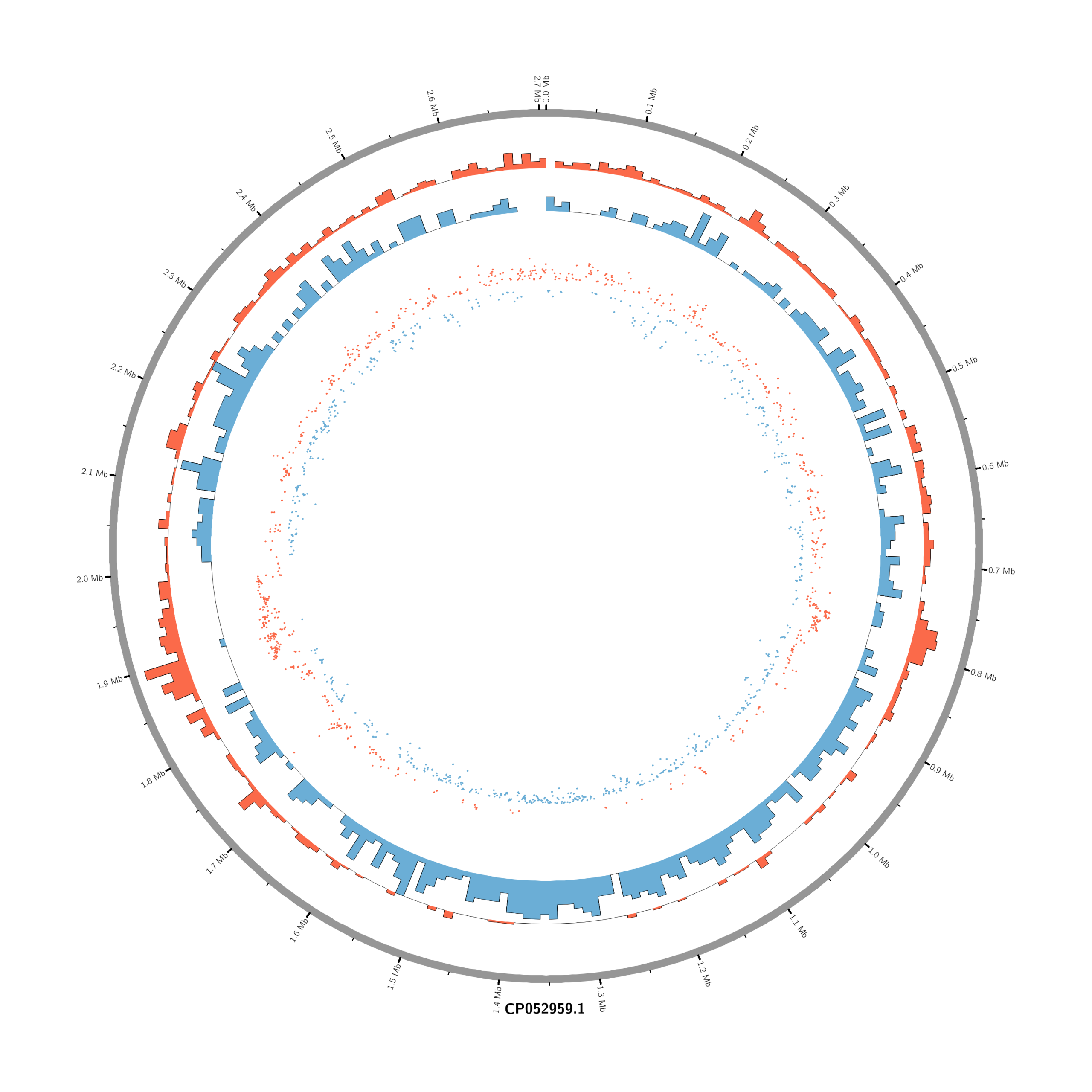
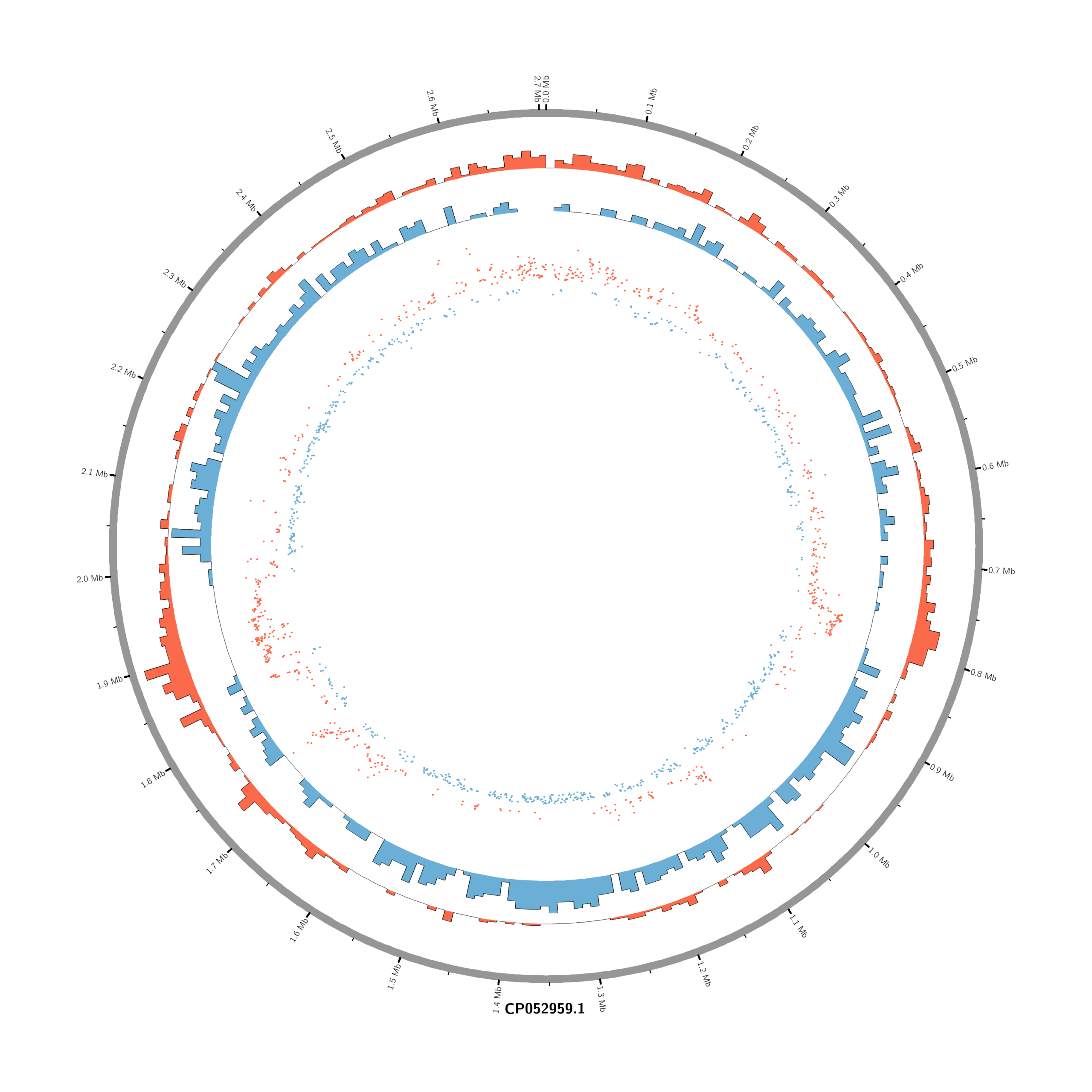
chr - CP052959.1 CP052959.1 0 2706926 grey karyotype = karyotype.txt
<ideogram>
<spacing>
default = 0.005r
</spacing>
radius = 0.80r
thickness = 20p
fill = yes
show_label = yes
label_radius = 1.05r
label_size = 30p
label_font = bold
label_parallel = yes
</ideogram>
# --- Wichtig: Schalter auf Top-Level, NICHT im
<ticks>-Block ---
show_ticks = yes
show_tick_labels = yes
<ticks>
# Starte direkt an der äußeren Ideogramm-Kante
radius = dims(ideogram,radius_outer)
orientation = out # Ticks nach außen zeichnen (oder 'in' für nach innen)
color = black
thickness = 2p
size = 8p
# kleine Ticks alle 100 kb, ohne Label
<tick>
spacing = 50000
size = 8p
thickness = 3p
color = black
show_label = no
</tick>
# große Ticks alle 500 kb, mit Label in Mb
<tick>
spacing = 100000
size = 12p
thickness = 5p
color = black
show_label = yes
label_size = 18p
label_offset = 6p
multiplier = 0.000001 # in Mb
format = %.1f
suffix = " Mb"
</tick>
</ticks>
<plots>
# Density of up-regulated genes
<plot>
show = yes
type = histogram
file = data/density_up.txt
r0 = 0.88r
r1 = 0.78r
fill_color = red
thickness = 1p
</plot>
# Density of down-regulated genes
<plot>
show = yes
type = histogram
file = data/density_down.txt
r0 = 0.78r
r1 = 0.68r
fill_color = blue
thickness = 1p
</plot>
# Scatter of individual significantly DE genes
<plot>
show = yes
type = scatter
file = data/genes_scatter.txt
r0 = 0.46r
r1 = 0.76r
glyph = circle
glyph_size = 5p
stroke_thickness = 0
min = -15
max = 15
<rules>
<rule>
condition = var(value) > 0
color = red
</rule>
<rule>
condition = var(value) < 0
color = blue
</rule>
</rules>
</plot>
</plots>
<image>
<<include etc/image.conf>>
</image>
<<include etc/colors_fonts_patterns.conf>>
<<include etc/housekeeping.conf>>Rscript make_circos_from_deseq.R
 ############################################################
 # make_circos_from_deseq.R
 #
 # - Read DESeq2 results (annotated CSV)
 # - Read BED annotation
 # - Merge by GeneID
 # - Classify genes (up / down / ns)
 # - Create Circos input files:
 #     * genes_scatter.txt
 #     * density_up.txt
 #     * density_down.txt
 # - Create annotated versions of the above
 # - Export annotated tables into one Excel workbook
 ############################################################

 ###############################
 # 0. Single parameter to set
 ###############################

 # Just change this line for each comparison:
 #comparison <- "Moxi_18h_vs_Untreated_18h"
 # e.g.
 #comparison <- "Mitomycin_18h_vs_Untreated_18h"
 #comparison <- "Mitomycin_8h_vs_Untreated_8h"
 #comparison <- "Moxi_8h_vs_Untreated_8h"
 #comparison <- "Mitomycin_4h_vs_Untreated_4h"
 comparison <- "Moxi_4h_vs_Untreated_4h"

 ###############################
 # 0. Derived settings
 ###############################

 # DESeq2 result file (annotated)
 deseq_file <- paste0(comparison, "-all_annotated.csv")

 # BED file with gene coordinates (constant for this genome)
 bed_file   <- "CP052959_m.bed"

 # Create a filesystem-friendly directory name from comparison
 safe_comp  <- gsub("[^A-Za-z0-9_]+", "_", comparison)

 # Output directory for Circos files (e.g. circos_Moxi_18h_vs_Untreated_18h)
 out_dir    <- paste0("circos_", safe_comp)

 # Thresholds for significance
 padj_cutoff <- 0.05
 lfc_cutoff  <- 1      # |log2FC| >= 1

 # Bin size for density in bp (e.g. 10000 = 10 kb)
 bin_size <- 10000

 # Comparison label for Excel / plots (human-readable)
 comparison_label <- comparison

 options(scipen = 999) # turn off scientific notation

 ###############################
 # 1. Setup & packages
 ###############################

 if (!dir.exists(out_dir)) dir.create(out_dir, showWarnings = FALSE)
 data_dir <- file.path(out_dir, "data")
 if (!dir.exists(data_dir)) dir.create(data_dir, showWarnings = FALSE)

 # openxlsx for Excel export
 if (!requireNamespace("openxlsx", quietly = TRUE)) {
 stop("Package 'openxlsx' is required. Please install it with install.packages('openxlsx').")
 }
 library(openxlsx)

 ###############################
 # 2. Read data
 ###############################

 message("Reading DESeq2 results from: ", deseq_file)
 deseq <- read.csv(deseq_file, stringsAsFactors = FALSE)

 # Check required columns in DESeq2 table
 required_cols <- c("GeneID", "log2FoldChange", "padj")
 if (!all(required_cols %in% colnames(deseq))) {
 stop("DESeq2 table must contain columns: ", paste(required_cols, collapse = ", "))
 }

 message("Reading BED annotation from: ", bed_file)
 bed_cols <- c("chr","start","end","gene_id","score",
             "strand","thickStart","thickEnd",
             "itemRgb","blockCount","blockSizes","blockStarts")

 annot <- read.table(
 bed_file,
 header = FALSE,
 sep = "\t",
 stringsAsFactors = FALSE,
 col.names = bed_cols
 )

 ###############################
 # 3. Merge DESeq2 + annotation
 ###############################

 # Match DESeq2 GeneID (e.g. "gene-HJI06_09365") to BED gene_id
 merged <- merge(
 deseq,
 annot[, c("chr", "start", "end", "gene_id")],
 by.x = "GeneID",
 by.y = "gene_id"
 )

 if (nrow(merged) == 0) {
 stop("No overlap between DESeq2 GeneID and BED gene_id.")
 }

 # Midpoint of each gene
 merged$mid <- round((merged$start + merged$end) / 2)

 ###############################
 # 4. Classify genes
 ###############################

 merged$regulation <- "ns"
 merged$regulation[merged$padj < padj_cutoff & merged$log2FoldChange >=  lfc_cutoff]  <- "up"
 merged$regulation[merged$padj < padj_cutoff & merged$log2FoldChange <= -lfc_cutoff] <- "down"

 table_reg <- table(merged$regulation)
 message("Regulation counts: ", paste(names(table_reg), table_reg, collapse = " | "))

 ###############################
 # 5. Scatter files (per-gene)
 ###############################

 scatter <- merged[merged$regulation != "ns", ]

 # Circos scatter input: chr  start  end  value
 scatter_file <- file.path(data_dir, "genes_scatter.txt")
 scatter_out  <- scatter[, c("chr", "mid", "mid", "log2FoldChange")]

 write.table(scatter_out,
             scatter_file,
             quote = FALSE, sep = "\t",
             row.names = FALSE, col.names = FALSE)

 message("Written Circos scatter file: ", scatter_file)

 # Annotated scatter for Excel / inspection
 scatter_annot <- scatter[, c(
 "chr",
 "mid",              # start
 "mid",              # end
 "log2FoldChange",
 "GeneID",
 "padj",
 "regulation"
 )]
 colnames(scatter_annot)[1:4] <- c("chr", "start", "end", "log2FoldChange")

 scatter_annot_file <- file.path(data_dir, "genes_scatter_annotated.tsv")
 write.table(scatter_annot,
             scatter_annot_file,
             quote = FALSE, sep = "\t",
             row.names = FALSE, col.names = TRUE)

 message("Written annotated scatter file: ", scatter_annot_file)

 ###############################
 # 6. Density function (bins)
 ###############################

 bin_chr <- function(df_chr, bin_size, direction = c("up", "down")) {
 direction <- match.arg(direction)

 chr_name <- df_chr$chr[1]
 max_pos  <- max(df_chr$mid)

 # number of bins
 n_bins <- ceiling((max_pos + 1) / bin_size)

 starts <- seq(0, by = bin_size, length.out = n_bins)
 ends   <- starts + bin_size

 # init counts & gene lists
 counts    <- integer(n_bins)
 gene_list <- vector("list", n_bins)

 df_dir <- df_chr[df_chr$regulation == direction, ]

 if (nrow(df_dir) > 0) {
     # bin index for each gene
     bin_index <- floor(df_dir$mid / bin_size) + 1
     bin_index[bin_index < 1]        <- 1
     bin_index[bin_index > n_bins]   <- n_bins

     # accumulate counts and GeneIDs
     for (i in seq_len(nrow(df_dir))) {
     idx <- bin_index[i]
     counts[idx] <- counts[idx] + 1L
     gene_list[[idx]] <- c(gene_list[[idx]], df_dir$GeneID[i])
     }
 }

 gene_ids <- vapply(
     gene_list,
     function(x) {
     if (length(x) == 0) "" else paste(unique(x), collapse = ";")
     },
     character(1)
 )

 data.frame(
     chr      = chr_name,
     start    = as.integer(starts),
     end      = as.integer(ends),
     value    = as.integer(counts),
     gene_ids = gene_ids,
     stringsAsFactors = FALSE
 )
 }

 ###############################
 # 7. Density up/down for all chromosomes
 ###############################

 chr_list <- split(merged, merged$chr)

 density_up_list   <- lapply(chr_list, bin_chr, bin_size = bin_size, direction = "up")
 density_down_list <- lapply(chr_list, bin_size = bin_size, FUN = bin_chr, direction = "down")

 density_up   <- do.call(rbind, density_up_list)
 density_down <- do.call(rbind, density_down_list)

 # Plain Circos input (no gene_ids)
 density_up_file   <- file.path(data_dir, "density_up.txt")
 density_down_file <- file.path(data_dir, "density_down.txt")

 write.table(density_up[, c("chr", "start", "end", "value")],
             density_up_file,
             quote = FALSE, sep = "\t",
             row.names = FALSE, col.names = FALSE)

 write.table(density_down[, c("chr", "start", "end", "value")],
             density_down_file,
             quote = FALSE, sep = "\t",
             row.names = FALSE, col.names = FALSE)

 message("Written Circos density files: ",
         density_up_file, " and ", density_down_file)

 # Annotated density files (with gene_ids)
 density_up_annot_file   <- file.path(data_dir, "density_up_annotated.tsv")
 density_down_annot_file <- file.path(data_dir, "density_down_annotated.tsv")

 write.table(density_up,
             density_up_annot_file,
             quote = FALSE, sep = "\t",
             row.names = FALSE, col.names = TRUE)

 write.table(density_down,
             density_down_annot_file,
             quote = FALSE, sep = "\t",
             row.names = FALSE, col.names = TRUE)

 message("Written annotated density files: ",
         density_up_annot_file, " and ", density_down_annot_file)

 ###############################
 # 8. Export annotated tables to Excel
 ###############################

 excel_file <- file.path(
 out_dir,
 paste0("circos_annotations_", comparison_label, ".xlsx")
 )

 wb <- createWorkbook()

 addWorksheet(wb, "scatter_points")
 writeData(wb, "scatter_points", scatter_annot)

 addWorksheet(wb, "density_up")
 writeData(wb, "density_up", density_up)

 addWorksheet(wb, "density_down")
 writeData(wb, "density_down", density_down)

 saveWorkbook(wb, excel_file, overwrite = TRUE)

 message("Excel workbook written to: ", excel_file)

 message("Done.")