-
Vorgabe
 #perform PCA analysis, Venn diagram analysis, as well as KEGG and GO annotations. We would also appreciate it if you could include CPM calculations for this dataset (gene_cpm_counts.xlsx). For comparative analysis, we are particularly interested in identifying DEGs between WT and ΔIJ across the different treatments and time points.

 I have already performed the six comparisons, using WT as the reference:

     ΔIJ-17 vs WT-17 – no treatment
     ΔIJ-24 vs WT-24 – no treatment
     preΔIJ-17 vs preWT-17 – Treatment A
     preΔIJ-24 vs preWT-24 – Treatment A
     0_5ΔIJ-17 vs 0_5WT-17 – Treatment B
     0_5ΔIJ-24 vs 0_5WT-24 – Treatment B

 To gain a deeper understanding of how the ∆adeIJ mutation influences response dynamics over time and under different stimuli, would you also be interested in the following additional comparisons?

 Within-strain treatment responses
 (to explore how each strain responds to treatments):

 WT:

     preWT-17 vs WT-17 → response to Treatment A at 17 h
     preWT-24 vs WT-24 → response to Treatment A at 24 h
     0_5WT-17 vs WT-17 → response to Treatment B at 17 h
     0_5WT-24 vs WT-24 → response to Treatment B at 24 h

 ∆adeIJ:

     preΔIJ-17 vs ΔIJ-17 → response to Treatment A at 17 h
     preΔIJ-24 vs ΔIJ-24 → response to Treatment A at 24 h
     0_5ΔIJ-17 vs ΔIJ-17 → response to Treatment B at 17 h
     0_5ΔIJ-24 vs ΔIJ-24 → response to Treatment B at 24 h

 Time-course comparisons
 (to investigate time-dependent changes within each condition):

     WT-24 vs WT-17
     ΔIJ-24 vs ΔIJ-17
     preWT-24 vs preWT-17
     preΔIJ-24 vs preΔIJ-17
     0_5WT-24 vs 0_5WT-17
     0_5ΔIJ-24 vs 0_5ΔIJ-17

 I reviewed the datasets again and noticed that there are no ∆adeAB samples included. Should we try to obtain ∆adeAB data from other datasets? However, I’m a bit concerned that batch effects might pose a challenge when integrating data from different datasets.

 > It is possible to analyze DEGs across various time points (17 and 24 h) and stimuli (treatment A and B, and without treatment) iswithin both the ∆adeIJ mutant and the WT strain as our phenotypic characterization of these strains across two times points and stimuli shows significant differences but the other mutant ∆adeAB (similar function as AdeIJ) shows no difference compared to WT, therefore we are wondering what's happened to ∆adeIJ.

 deltaIJ_17, WT_17 – ΔadeIJ and wildtype strains w/o exposure at 17 h (No treatment)
 deltaIJ_24, WT_24 – ΔadeIJ and wildtype strains w/o exposure at 24 h (No treatment)
 pre_deltaIJ_17, pre_WT_17 – ΔadeIJ and wildtype strains with 1 exposure at 17 h (Treatment A)
 pre_deltaIJ_24, pre_WT_24 – ΔadeIJ and wildtype strains with 1 exposure at 24 h (Treatment A)
 0_5_deltaIJ_17, 0_5_WT_17 – ΔadeIJ and wildtype strains with 2 exposure at 17 h (Treatment B)
 0_5_deltaIJ_24, 0_5_WT_24 – ΔadeIJ and wildtype strains with 2 exposure at 24 h (Treatment B)
-
Preparing raw data
 mkdir raw_data; cd raw_data
 ln -s ../RSMR00204/X101SC25062155-Z01/X101SC25062155-Z01-J001/01.RawData/WT-17-1/WT-17-1_1.fq.gz WT-17-r1_R1.fq.gz
 ln -s ../RSMR00204/X101SC25062155-Z01/X101SC25062155-Z01-J001/01.RawData/WT-17-1/WT-17-1_2.fq.gz WT-17-r1_R2.fq.gz
 ln -s ../RSMR00204/X101SC25062155-Z01/X101SC25062155-Z01-J001/01.RawData/WT-17-2/WT-17-2_1.fq.gz WT-17-r2_R1.fq.gz
 ln -s ../RSMR00204/X101SC25062155-Z01/X101SC25062155-Z01-J001/01.RawData/WT-17-2/WT-17-2_2.fq.gz WT-17-r2_R2.fq.gz
 ln -s ../RSMR00204/X101SC25062155-Z01/X101SC25062155-Z01-J001/01.RawData/WT-17-3/WT-17-3_1.fq.gz WT-17-r3_R1.fq.gz
 ln -s ../RSMR00204/X101SC25062155-Z01/X101SC25062155-Z01-J001/01.RawData/WT-17-3/WT-17-3_2.fq.gz WT-17-r3_R2.fq.gz
 ln -s ../RSMR00204/X101SC25062155-Z01/X101SC25062155-Z01-J001/01.RawData/WT-24-1/WT-24-1_1.fq.gz WT-24-r1_R1.fq.gz
 ln -s ../RSMR00204/X101SC25062155-Z01/X101SC25062155-Z01-J001/01.RawData/WT-24-1/WT-24-1_2.fq.gz WT-24-r1_R2.fq.gz
 ln -s ../RSMR00204/X101SC25062155-Z01/X101SC25062155-Z01-J001/01.RawData/WT-24-2/WT-24-2_1.fq.gz WT-24-r2_R1.fq.gz
 ln -s ../RSMR00204/X101SC25062155-Z01/X101SC25062155-Z01-J001/01.RawData/WT-24-2/WT-24-2_2.fq.gz WT-24-r2_R2.fq.gz
 ln -s ../RSMR00204/X101SC25062155-Z01/X101SC25062155-Z01-J001/01.RawData/WT-24-3/WT-24-3_1.fq.gz WT-24-r3_R1.fq.gz
 ln -s ../RSMR00204/X101SC25062155-Z01/X101SC25062155-Z01-J001/01.RawData/WT-24-3/WT-24-3_2.fq.gz WT-24-r3_R2.fq.gz
 ln -s ../RSMR00204/X101SC25062155-Z01/X101SC25062155-Z01-J001/01.RawData/ΔIJ-17-1/ΔIJ-17-1_1.fq.gz deltaIJ-17-r1_R1.fq.gz
 ln -s ../RSMR00204/X101SC25062155-Z01/X101SC25062155-Z01-J001/01.RawData/ΔIJ-17-1/ΔIJ-17-1_2.fq.gz deltaIJ-17-r1_R2.fq.gz
 ln -s ../RSMR00204/X101SC25062155-Z01/X101SC25062155-Z01-J001/01.RawData/ΔIJ-17-2/ΔIJ-17-2_1.fq.gz deltaIJ-17-r2_R1.fq.gz
 ln -s ../RSMR00204/X101SC25062155-Z01/X101SC25062155-Z01-J001/01.RawData/ΔIJ-17-2/ΔIJ-17-2_2.fq.gz deltaIJ-17-r2_R2.fq.gz
 ln -s ../RSMR00204/X101SC25062155-Z01/X101SC25062155-Z01-J001/01.RawData/ΔIJ-17-3/ΔIJ-17-3_1.fq.gz deltaIJ-17-r3_R1.fq.gz
 ln -s ../RSMR00204/X101SC25062155-Z01/X101SC25062155-Z01-J001/01.RawData/ΔIJ-17-3/ΔIJ-17-3_2.fq.gz deltaIJ-17-r3_R2.fq.gz
 ln -s ../RSMR00204/X101SC25062155-Z01/X101SC25062155-Z01-J001/01.RawData/ΔIJ-24-1/ΔIJ-24-1_1.fq.gz deltaIJ-24-r1_R1.fq.gz
 ln -s ../RSMR00204/X101SC25062155-Z01/X101SC25062155-Z01-J001/01.RawData/ΔIJ-24-1/ΔIJ-24-1_2.fq.gz deltaIJ-24-r1_R2.fq.gz
 ln -s ../RSMR00204/X101SC25062155-Z01/X101SC25062155-Z01-J001/01.RawData/ΔIJ-24-2/ΔIJ-24-2_1.fq.gz deltaIJ-24-r2_R1.fq.gz
 ln -s ../RSMR00204/X101SC25062155-Z01/X101SC25062155-Z01-J001/01.RawData/ΔIJ-24-2/ΔIJ-24-2_2.fq.gz deltaIJ-24-r2_R2.fq.gz
 ln -s ../RSMR00204/X101SC25062155-Z01/X101SC25062155-Z01-J001/01.RawData/ΔIJ-24-3/ΔIJ-24-3_1.fq.gz deltaIJ-24-r3_R1.fq.gz
 ln -s ../RSMR00204/X101SC25062155-Z01/X101SC25062155-Z01-J001/01.RawData/ΔIJ-24-3/ΔIJ-24-3_2.fq.gz deltaIJ-24-r3_R2.fq.gz

 ln -s ../RSMR00204/X101SC25062155-Z01/X101SC25062155-Z01-J001/01.RawData/preWT-17-1/preWT-17-1_1.fq.gz pre_WT-17-r1_R1.fq.gz
 ln -s ../RSMR00204/X101SC25062155-Z01/X101SC25062155-Z01-J001/01.RawData/preWT-17-1/preWT-17-1_2.fq.gz pre_WT-17-r1_R2.fq.gz
 ln -s ../RSMR00204/X101SC25062155-Z01/X101SC25062155-Z01-J001/01.RawData/preWT-17-2/preWT-17-2_1.fq.gz pre_WT-17-r2_R1.fq.gz
 ln -s ../RSMR00204/X101SC25062155-Z01/X101SC25062155-Z01-J001/01.RawData/preWT-17-2/preWT-17-2_2.fq.gz pre_WT-17-r2_R2.fq.gz
 ln -s ../RSMR00204/X101SC25062155-Z01/X101SC25062155-Z01-J001/01.RawData/preWT-17-3/preWT-17-3_1.fq.gz pre_WT-17-r3_R1.fq.gz
 ln -s ../RSMR00204/X101SC25062155-Z01/X101SC25062155-Z01-J001/01.RawData/preWT-17-3/preWT-17-3_2.fq.gz pre_WT-17-r3_R2.fq.gz
 ln -s ../RSMR00204/X101SC25062155-Z01/X101SC25062155-Z01-J001/01.RawData/preWT-24-1/preWT-24-1_1.fq.gz pre_WT-24-r1_R1.fq.gz
 ln -s ../RSMR00204/X101SC25062155-Z01/X101SC25062155-Z01-J001/01.RawData/preWT-24-1/preWT-24-1_2.fq.gz pre_WT-24-r1_R2.fq.gz
 ln -s ../RSMR00204/X101SC25062155-Z01/X101SC25062155-Z01-J001/01.RawData/preWT-24-2/preWT-24-2_1.fq.gz pre_WT-24-r2_R1.fq.gz
 ln -s ../RSMR00204/X101SC25062155-Z01/X101SC25062155-Z01-J001/01.RawData/preWT-24-2/preWT-24-2_2.fq.gz pre_WT-24-r2_R2.fq.gz
 ln -s ../RSMR00204/X101SC25062155-Z01/X101SC25062155-Z01-J001/01.RawData/preWT-24-3/preWT-24-3_1.fq.gz pre_WT-24-r3_R1.fq.gz
 ln -s ../RSMR00204/X101SC25062155-Z01/X101SC25062155-Z01-J001/01.RawData/preWT-24-3/preWT-24-3_2.fq.gz pre_WT-24-r3_R2.fq.gz
 ln -s ../RSMR00204/X101SC25062155-Z01/X101SC25062155-Z01-J001/01.RawData/preΔIJ-17-1/preΔIJ-17-1_1.fq.gz pre_deltaIJ-17-r1_R1.fq.gz
 ln -s ../RSMR00204/X101SC25062155-Z01/X101SC25062155-Z01-J001/01.RawData/preΔIJ-17-1/preΔIJ-17-1_2.fq.gz pre_deltaIJ-17-r1_R2.fq.gz
 ln -s ../RSMR00204/X101SC25062155-Z01/X101SC25062155-Z01-J001/01.RawData/preΔIJ-17-2/preΔIJ-17-2_1.fq.gz pre_deltaIJ-17-r2_R1.fq.gz
 ln -s ../RSMR00204/X101SC25062155-Z01/X101SC25062155-Z01-J001/01.RawData/preΔIJ-17-2/preΔIJ-17-2_2.fq.gz pre_deltaIJ-17-r2_R2.fq.gz
 ln -s ../RSMR00204/X101SC25062155-Z01/X101SC25062155-Z01-J001/01.RawData/preΔIJ-17-3/preΔIJ-17-3_1.fq.gz pre_deltaIJ-17-r3_R1.fq.gz
 ln -s ../RSMR00204/X101SC25062155-Z01/X101SC25062155-Z01-J001/01.RawData/preΔIJ-17-3/preΔIJ-17-3_2.fq.gz pre_deltaIJ-17-r3_R2.fq.gz
 ln -s ../RSMR00204/X101SC25062155-Z01/X101SC25062155-Z01-J001/01.RawData/preΔIJ-24-1/preΔIJ-24-1_1.fq.gz pre_deltaIJ-24-r1_R1.fq.gz
 ln -s ../RSMR00204/X101SC25062155-Z01/X101SC25062155-Z01-J001/01.RawData/preΔIJ-24-1/preΔIJ-24-1_2.fq.gz pre_deltaIJ-24-r1_R2.fq.gz
 ln -s ../RSMR00204/X101SC25062155-Z01/X101SC25062155-Z01-J001/01.RawData/preΔIJ-24-2/preΔIJ-24-2_1.fq.gz pre_deltaIJ-24-r2_R1.fq.gz
 ln -s ../RSMR00204/X101SC25062155-Z01/X101SC25062155-Z01-J001/01.RawData/preΔIJ-24-2/preΔIJ-24-2_2.fq.gz pre_deltaIJ-24-r2_R2.fq.gz
 ln -s ../RSMR00204/X101SC25062155-Z01/X101SC25062155-Z01-J001/01.RawData/preΔIJ-24-3/preΔIJ-24-3_1.fq.gz pre_deltaIJ-24-r3_R1.fq.gz
 ln -s ../RSMR00204/X101SC25062155-Z01/X101SC25062155-Z01-J001/01.RawData/preΔIJ-24-3/preΔIJ-24-3_2.fq.gz pre_deltaIJ-24-r3_R2.fq.gz

 ln -s ../RSMR00204/X101SC25062155-Z01/X101SC25062155-Z01-J001/01.RawData/WT0_5-17-1/WT0_5-17-1_1.fq.gz 0_5_WT-17-r1_R1.fq.gz
 ln -s ../RSMR00204/X101SC25062155-Z01/X101SC25062155-Z01-J001/01.RawData/WT0_5-17-1/WT0_5-17-1_2.fq.gz 0_5_WT-17-r1_R2.fq.gz
 ln -s ../RSMR00204/X101SC25062155-Z01/X101SC25062155-Z01-J001/01.RawData/WT0_5-17-2/WT0_5-17-2_1.fq.gz 0_5_WT-17-r2_R1.fq.gz
 ln -s ../RSMR00204/X101SC25062155-Z01/X101SC25062155-Z01-J001/01.RawData/WT0_5-17-2/WT0_5-17-2_2.fq.gz 0_5_WT-17-r2_R2.fq.gz
 ln -s ../RSMR00204/X101SC25062155-Z01/X101SC25062155-Z01-J001/01.RawData/WT0_5-17-3/WT0_5-17-3_1.fq.gz 0_5_WT-17-r3_R1.fq.gz
 ln -s ../RSMR00204/X101SC25062155-Z01/X101SC25062155-Z01-J001/01.RawData/WT0_5-17-3/WT0_5-17-3_2.fq.gz 0_5_WT-17-r3_R2.fq.gz
 ln -s ../RSMR00204/X101SC25062155-Z01/X101SC25062155-Z01-J001/01.RawData/WT0_5-24-1/WT0_5-24-1_1.fq.gz 0_5_WT-24-r1_R1.fq.gz
 ln -s ../RSMR00204/X101SC25062155-Z01/X101SC25062155-Z01-J001/01.RawData/WT0_5-24-1/WT0_5-24-1_2.fq.gz 0_5_WT-24-r1_R2.fq.gz
 ln -s ../RSMR00204/X101SC25062155-Z01/X101SC25062155-Z01-J001/01.RawData/WT0_5-24-2/WT0_5-24-2_1.fq.gz 0_5_WT-24-r2_R1.fq.gz
 ln -s ../RSMR00204/X101SC25062155-Z01/X101SC25062155-Z01-J001/01.RawData/WT0_5-24-2/WT0_5-24-2_2.fq.gz 0_5_WT-24-r2_R2.fq.gz
 ln -s ../RSMR00204/X101SC25062155-Z01/X101SC25062155-Z01-J001/01.RawData/WT0_5-24-3/WT0_5-24-3_1.fq.gz 0_5_WT-24-r3_R1.fq.gz
 ln -s ../RSMR00204/X101SC25062155-Z01/X101SC25062155-Z01-J001/01.RawData/WT0_5-24-3/WT0_5-24-3_2.fq.gz 0_5_WT-24-r3_R2.fq.gz
 ln -s ../RSMR00204/X101SC25062155-Z01/X101SC25062155-Z01-J001/01.RawData/0_5ΔIJ-17-1/0_5ΔIJ-17-1_1.fq.gz 0_5_deltaIJ-17-r1_R1.fq.gz
 ln -s ../RSMR00204/X101SC25062155-Z01/X101SC25062155-Z01-J001/01.RawData/0_5ΔIJ-17-1/0_5ΔIJ-17-1_2.fq.gz 0_5_deltaIJ-17-r1_R2.fq.gz
 ln -s ../RSMR00204/X101SC25062155-Z01/X101SC25062155-Z01-J001/01.RawData/0_5ΔIJ-17-2/0_5ΔIJ-17-2_1.fq.gz 0_5_deltaIJ-17-r2_R1.fq.gz
 ln -s ../RSMR00204/X101SC25062155-Z01/X101SC25062155-Z01-J001/01.RawData/0_5ΔIJ-17-2/0_5ΔIJ-17-2_2.fq.gz 0_5_deltaIJ-17-r2_R2.fq.gz
 ln -s ../RSMR00204/X101SC25062155-Z01/X101SC25062155-Z01-J001/01.RawData/0_5ΔIJ-17-3/0_5ΔIJ-17-3_1.fq.gz 0_5_deltaIJ-17-r3_R1.fq.gz
 ln -s ../RSMR00204/X101SC25062155-Z01/X101SC25062155-Z01-J001/01.RawData/0_5ΔIJ-17-3/0_5ΔIJ-17-3_2.fq.gz 0_5_deltaIJ-17-r3_R2.fq.gz
 ln -s ../RSMR00204/X101SC25062155-Z01/X101SC25062155-Z01-J001/01.RawData/0_5ΔIJ-24-1/0_5ΔIJ-24-1_1.fq.gz 0_5_deltaIJ-24-r1_R1.fq.gz
 ln -s ../RSMR00204/X101SC25062155-Z01/X101SC25062155-Z01-J001/01.RawData/0_5ΔIJ-24-1/0_5ΔIJ-24-1_2.fq.gz 0_5_deltaIJ-24-r1_R2.fq.gz
 ln -s ../RSMR00204/X101SC25062155-Z01/X101SC25062155-Z01-J001/01.RawData/0_5ΔIJ-24-2/0_5ΔIJ-24-2_1.fq.gz 0_5_deltaIJ-24-r2_R1.fq.gz
 ln -s ../RSMR00204/X101SC25062155-Z01/X101SC25062155-Z01-J001/01.RawData/0_5ΔIJ-24-2/0_5ΔIJ-24-2_2.fq.gz 0_5_deltaIJ-24-r2_R2.fq.gz
 ln -s ../RSMR00204/X101SC25062155-Z01/X101SC25062155-Z01-J001/01.RawData/0_5ΔIJ-24-3/0_5ΔIJ-24-3_1.fq.gz 0_5_deltaIJ-24-r3_R1.fq.gz
 ln -s ../RSMR00204/X101SC25062155-Z01/X101SC25062155-Z01-J001/01.RawData/0_5ΔIJ-24-3/0_5ΔIJ-24-3_2.fq.gz 0_5_deltaIJ-24-r3_R2.fq.gz
-
(Done) Downloading CP059040.fasta and CP059040.gff from GenBank
-
Preparing the directory trimmed
 mkdir trimmed trimmed_unpaired;
 for sample_id in WT-17-r1 WT-17-r2 WT-17-r3 WT-24-r1 WT-24-r2 WT-24-r3 deltaIJ-17-r1 deltaIJ-17-r2 deltaIJ-17-r3 deltaIJ-24-r1 deltaIJ-24-r2 deltaIJ-24-r3  pre_WT-17-r1 pre_WT-17-r2 pre_WT-17-r3 pre_WT-24-r1 pre_WT-24-r2 pre_WT-24-r3 pre_deltaIJ-17-r1 pre_deltaIJ-17-r2 pre_deltaIJ-17-r3 pre_deltaIJ-24-r1 pre_deltaIJ-24-r2 pre_deltaIJ-24-r3  0_5_WT-17-r1 0_5_WT-17-r2 0_5_WT-17-r3 0_5_WT-24-r1 0_5_WT-24-r2 0_5_WT-24-r3 0_5_deltaIJ-17-r1 0_5_deltaIJ-17-r2 0_5_deltaIJ-17-r3 0_5_deltaIJ-24-r1 0_5_deltaIJ-24-r2 0_5_deltaIJ-24-r3; do \
         java -jar /home/jhuang/Tools/Trimmomatic-0.36/trimmomatic-0.36.jar PE -threads 100 raw_data/${sample_id}_R1.fq.gz raw_data/${sample_id}_R2.fq.gz trimmed/${sample_id}_R1.fq.gz trimmed_unpaired/${sample_id}_R1.fq.gz trimmed/${sample_id}_R2.fq.gz trimmed_unpaired/${sample_id}_R2.fq.gz ILLUMINACLIP:/home/jhuang/Tools/Trimmomatic-0.36/adapters/TruSeq3-PE-2.fa:2:30:10:8:TRUE LEADING:3 TRAILING:3 SLIDINGWINDOW:4:15 MINLEN:36 AVGQUAL:20; done 2> trimmomatic_pe.log;
 done
-
Preparing samplesheet.csv
 sample,fastq_1,fastq_2,strandedness
 WT_17_r1,WT-17-r1_R1.fq.gz,WT-17-r1_R2.fq.gz,auto
 WT_17_r2,WT-17-r2_R1.fq.gz,WT-17-r2_R2.fq.gz,auto
 WT_17_r3,WT-17-r3_R1.fq.gz,WT-17-r3_R2.fq.gz,auto
 WT_24_r1,WT-24-r1_R1.fq.gz,WT-24-r1_R2.fq.gz,auto
 WT_24_r2,WT-24-r2_R1.fq.gz,WT-24-r2_R2.fq.gz,auto
 WT_24_r3,WT-24-r3_R1.fq.gz,WT-24-r3_R2.fq.gz,auto
 deltaIJ_17_r1,deltaIJ-17-r1_R1.fq.gz,deltaIJ-17-r1_R2.fq.gz,auto
 deltaIJ_17_r2,deltaIJ-17-r2_R1.fq.gz,deltaIJ-17-r2_R2.fq.gz,auto
 deltaIJ_17_r3,deltaIJ-17-r3_R1.fq.gz,deltaIJ-17-r3_R2.fq.gz,auto
 deltaIJ_24_r1,deltaIJ-24-r1_R1.fq.gz,deltaIJ-24-r1_R2.fq.gz,auto
 deltaIJ_24_r2,deltaIJ-24-r2_R1.fq.gz,deltaIJ-24-r2_R2.fq.gz,auto
 deltaIJ_24_r3,deltaIJ-24-r3_R1.fq.gz,deltaIJ-24-r3_R2.fq.gz,auto
 pre_WT_17_r1,pre_WT-17-r1_R1.fq.gz,pre_WT-17-r1_R2.fq.gz,auto
 pre_WT_17_r2,pre_WT-17-r2_R1.fq.gz,pre_WT-17-r2_R2.fq.gz,auto
 pre_WT_17_r3,pre_WT-17-r3_R1.fq.gz,pre_WT-17-r3_R2.fq.gz,auto
 pre_WT_24_r1,pre_WT-24-r1_R1.fq.gz,pre_WT-24-r1_R2.fq.gz,auto
 pre_WT_24_r2,pre_WT-24-r2_R1.fq.gz,pre_WT-24-r2_R2.fq.gz,auto
 pre_WT_24_r3,pre_WT-24-r3_R1.fq.gz,pre_WT-24-r3_R2.fq.gz,auto
 pre_deltaIJ_17_r1,pre_deltaIJ-17-r1_R1.fq.gz,pre_deltaIJ-17-r1_R2.fq.gz,auto
 pre_deltaIJ_17_r2,pre_deltaIJ-17-r2_R1.fq.gz,pre_deltaIJ-17-r2_R2.fq.gz,auto
 pre_deltaIJ_17_r3,pre_deltaIJ-17-r3_R1.fq.gz,pre_deltaIJ-17-r3_R2.fq.gz,auto
 pre_deltaIJ_24_r1,pre_deltaIJ-24-r1_R1.fq.gz,pre_deltaIJ-24-r1_R2.fq.gz,auto
 pre_deltaIJ_24_r2,pre_deltaIJ-24-r2_R1.fq.gz,pre_deltaIJ-24-r2_R2.fq.gz,auto
 pre_deltaIJ_24_r3,pre_deltaIJ-24-r3_R1.fq.gz,pre_deltaIJ-24-r3_R2.fq.gz,auto
 0_5_WT_17_r1,0_5_WT-17-r1_R1.fq.gz,0_5_WT-17-r1_R2.fq.gz,auto
 0_5_WT_17_r2,0_5_WT-17-r2_R1.fq.gz,0_5_WT-17-r2_R2.fq.gz,auto
 0_5_WT_17_r3,0_5_WT-17-r3_R1.fq.gz,0_5_WT-17-r3_R2.fq.gz,auto
 0_5_WT_24_r1,0_5_WT-24-r1_R1.fq.gz,0_5_WT-24-r1_R2.fq.gz,auto
 0_5_WT_24_r2,0_5_WT-24-r2_R1.fq.gz,0_5_WT-24-r2_R2.fq.gz,auto
 0_5_WT_24_r3,0_5_WT-24-r3_R1.fq.gz,0_5_WT-24-r3_R2.fq.gz,auto
 0_5_deltaIJ_17_r1,0_5_deltaIJ-17-r1_R1.fq.gz,0_5_deltaIJ-17-r1_R2.fq.gz,auto
 0_5_deltaIJ_17_r2,0_5_deltaIJ-17-r2_R1.fq.gz,0_5_deltaIJ-17-r2_R2.fq.gz,auto
 0_5_deltaIJ_17_r3,0_5_deltaIJ-17-r3_R1.fq.gz,0_5_deltaIJ-17-r3_R2.fq.gz,auto
 0_5_deltaIJ_24_r1,0_5_deltaIJ-24-r1_R1.fq.gz,0_5_deltaIJ-24-r1_R2.fq.gz,auto
 0_5_deltaIJ_24_r2,0_5_deltaIJ-24-r2_R1.fq.gz,0_5_deltaIJ-24-r2_R2.fq.gz,auto
 0_5_deltaIJ_24_r3,0_5_deltaIJ-24-r3_R1.fq.gz,0_5_deltaIJ-24-r3_R2.fq.gz,auto
-
nextflow run
 #Example1: http://xgenes.com/article/article-content/157/prepare-virus-gtf-for-nextflow-run/

 docker pull nfcore/rnaseq
 ln -s /home/jhuang/Tools/nf-core-rnaseq-3.12.0/ rnaseq

 #Default: --gtf_group_features 'gene_id'  --gtf_extra_attributes 'gene_name' --featurecounts_group_type 'gene_biotype' --featurecounts_feature_type 'exon'
 #(host_env) !NOT_WORKING! jhuang@WS-2290C:~/DATA/Data_Tam_RNAseq_2024$ /usr/local/bin/nextflow run rnaseq/main.nf --input samplesheet.csv --outdir results    --fasta "/home/jhuang/DATA/Data_Tam_RNAseq_2024/CP059040.fasta" --gff "/home/jhuang/DATA/Data_Tam_RNAseq_2024/CP059040.gff"        -profile docker -resume  --max_cpus 55 --max_memory 512.GB --max_time 2400.h    --save_align_intermeds --save_unaligned --save_reference    --aligner 'star_salmon'    --gtf_group_features 'gene_id'  --gtf_extra_attributes 'gene_name' --featurecounts_group_type 'gene_biotype' --featurecounts_feature_type 'transcript'

 # -- DEBUG_1 (CDS --> exon in CP059040.gff) --
 #Checking the record (see below) in results/genome/CP059040.gtf
 #In ./results/genome/CP059040.gtf e.g. "CP059040.1      Genbank transcript      1       1398    .       +       .       transcript_id "gene-H0N29_00005"; gene_id "gene-H0N29_00005"; gene_name "dnaA"; Name "dnaA"; gbkey "Gene"; gene "dnaA"; gene_biotype "protein_coding"; locus_tag "H0N29_00005";"
 #--featurecounts_feature_type 'transcript' returns only the tRNA results
 #Since the tRNA records have "transcript and exon". In gene records, we have "transcript and CDS". replace the CDS with exon

 grep -P "\texon\t" CP059040.gff | sort | wc -l    #96
 grep -P "cmsearch\texon\t" CP059040.gff | wc -l    #=10  ignal recognition particle sRNA small typ, transfer-messenger RNA, 5S ribosomal RNA
 grep -P "Genbank\texon\t" CP059040.gff | wc -l    #=12  16S and 23S ribosomal RNA
 grep -P "tRNAscan-SE\texon\t" CP059040.gff | wc -l    #tRNA 74
 wc -l star_salmon/AUM_r3/quant.genes.sf  #--featurecounts_feature_type 'transcript' results in 96 records!

 grep -P "\tCDS\t" CP059040.gff | wc -l  #3701
 sed 's/\tCDS\t/\texon\t/g' CP059040.gff > CP059040_m.gff
 grep -P "\texon\t" CP059040_m.gff | sort | wc -l  #3797

 # -- DEBUG_2: combination of 'CP059040_m.gff' and 'exon' results in ERROR, using 'transcript' instead!
 --gff "/home/jhuang/DATA/Data_Tam_RNAseq_2024/CP059040_m.gff" --featurecounts_feature_type 'transcript'

 # ---- SUCCESSFUL with directly downloaded gff3 and fasta from NCBI using docker after replacing 'CDS' with 'exon' ----
 mv trimmed/*.fq.gz .; rmdir trimmed
 (host_env) /usr/local/bin/nextflow run rnaseq/main.nf --input samplesheet.csv --outdir results    --fasta "/home/jhuang/DATA/Data_Tam_RNAseq_2024_AUM_MHB_Urine_ATCC19606/CP059040.fasta" --gff "/home/jhuang/DATA/Data_Tam_RNAseq_2024_AUM_MHB_Urine_ATCC19606/CP059040_m.gff"        -profile docker -resume  --max_cpus 90 --max_memory 900.GB --max_time 2400.h    --save_align_intermeds --save_unaligned --save_reference    --aligner 'star_salmon'    --gtf_group_features 'gene_id'  --gtf_extra_attributes 'gene_name' --featurecounts_group_type 'gene_biotype' --featurecounts_feature_type 'transcript'

 # -- DEBUG_3: make sure the header of fasta is the same to the *_m.gff file
-
Prepare counts_fixed by hand: delete all “””, “gene-“, replace , to ‘\t’.
 cp ./results/star_salmon/gene_raw_counts.csv counts.tsv

 #keep only gene_id
 cut -f1 -d',' counts.tsv > f1
 cut -f3- -d',' counts.tsv > f3_
 paste -d',' f1 f3_ > counts_fixed.tsv

 Rscript rna_timecourse_bacteria.R \
   --counts counts_fixed.tsv \
   --samples samples.tsv \
   --condition_col condition \
   --time_col time_h \
   --emapper ~/DATA/Data_Tam_RNAseq_2024_AUM_MHB_Urine_ATCC19606/eggnog_out.emapper.annotations.txt \
   --volcano_csvs contrasts/ctrl_vs_treat.csv \
   --outdir results_bacteria

 #Delete the repliate 2 of ΔadeIJ_two_17 and repliate 1 of ΔadeIJ_two_24 are outlier.
 paste -d$'\t' f1_32 f34 f36_ > counts_fixed_2.tsv

 Rscript rna_timecourse_bacteria.R \
   --counts counts_fixed_2.tsv \
   --samples samples_2.tsv \
   --condition_col condition \
   --time_col time_h \
   --emapper ~/DATA/Data_Tam_RNAseq_2024_AUM_MHB_Urine_ATCC19606/eggnog_out.emapper.annotations.txt \
   --volcano_csvs contrasts/ctrl_vs_treat.csv \
   --outdir results_bacteria_2
-
Import data and pca-plot
 #mamba activate r_env

 #install.packages("ggfun")
 # Import the required libraries
 library("AnnotationDbi")
 library("clusterProfiler")
 library("ReactomePA")
 library(gplots)
 library(tximport)
 library(DESeq2)
 #library("org.Hs.eg.db")
 library(dplyr)
 library(tidyverse)
 #install.packages("devtools")
 #devtools::install_version("gtable", version = "0.3.0")
 library(gplots)
 library("RColorBrewer")
 #install.packages("ggrepel")
 library("ggrepel")
 # install.packages("openxlsx")
 library(openxlsx)
 library(EnhancedVolcano)
 library(DESeq2)
 library(edgeR)

 setwd("~/DATA/Data_Tam_RNAseq_2025_subMIC_exposure_ATCC19606/results/star_salmon")
 # Define paths to your Salmon output quantification files
 files <- c("WT_17_r1" = "./WT_17_r1/quant.sf",
            "WT_17_r2" = "./WT_17_r2/quant.sf",
            "WT_17_r3" = "./WT_17_r3/quant.sf",
            "WT_24_r1" = "./WT_24_r1/quant.sf",
            "WT_24_r2" = "./WT_24_r2/quant.sf",
            "WT_24_r3" = "./WT_24_r3/quant.sf",
            "deltaIJ_17_r1" = "./deltaIJ_17_r1/quant.sf",
            "deltaIJ_17_r2" = "./deltaIJ_17_r2/quant.sf",
            "deltaIJ_17_r3" = "./deltaIJ_17_r3/quant.sf",
            "deltaIJ_24_r1" = "./deltaIJ_24_r1/quant.sf",
            "deltaIJ_24_r2" = "./deltaIJ_24_r2/quant.sf",
            "deltaIJ_24_r3" = "./deltaIJ_24_r3/quant.sf",
            "pre_WT_17_r1" = "./pre_WT_17_r1/quant.sf",
            "pre_WT_17_r2" = "./pre_WT_17_r2/quant.sf",
            "pre_WT_17_r3" = "./pre_WT_17_r3/quant.sf",
            "pre_WT_24_r1" = "./pre_WT_24_r1/quant.sf",
            "pre_WT_24_r2" = "./pre_WT_24_r2/quant.sf",
            "pre_WT_24_r3" = "./pre_WT_24_r3/quant.sf",
            "pre_deltaIJ_17_r1" = "./pre_deltaIJ_17_r1/quant.sf",
            "pre_deltaIJ_17_r2" = "./pre_deltaIJ_17_r2/quant.sf",
            "pre_deltaIJ_17_r3" = "./pre_deltaIJ_17_r3/quant.sf",
            "pre_deltaIJ_24_r1" = "./pre_deltaIJ_24_r1/quant.sf",
            "pre_deltaIJ_24_r2" = "./pre_deltaIJ_24_r2/quant.sf",
            "pre_deltaIJ_24_r3" = "./pre_deltaIJ_24_r3/quant.sf",
            "0_5_WT_17_r1" = "./0_5_WT_17_r1/quant.sf",
            "0_5_WT_17_r2" = "./0_5_WT_17_r2/quant.sf",
            "0_5_WT_17_r3" = "./0_5_WT_17_r3/quant.sf",
            "0_5_WT_24_r1" = "./0_5_WT_24_r1/quant.sf",
            "0_5_WT_24_r2" = "./0_5_WT_24_r2/quant.sf",
            "0_5_WT_24_r3" = "./0_5_WT_24_r3/quant.sf",
            "0_5_deltaIJ_17_r1" = "./0_5_deltaIJ_17_r1/quant.sf",
            "0_5_deltaIJ_17_r2" = "./0_5_deltaIJ_17_r2/quant.sf",
            "0_5_deltaIJ_17_r3" = "./0_5_deltaIJ_17_r3/quant.sf",
            "0_5_deltaIJ_24_r1" = "./0_5_deltaIJ_24_r1/quant.sf",
            "0_5_deltaIJ_24_r2" = "./0_5_deltaIJ_24_r2/quant.sf",
            "0_5_deltaIJ_24_r3" = "./0_5_deltaIJ_24_r3/quant.sf")
 # Import the transcript abundance data with tximport
 txi <- tximport(files, type = "salmon", txIn = TRUE, txOut = TRUE)
 # Define the replicates and condition of the samples
 replicate <- factor(c("r1", "r2", "r3",  "r1", "r2", "r3", "r1", "r2", "r3", "r1", "r2", "r3",     "r1", "r2", "r3", "r1", "r2", "r3", "r1", "r2", "r3", "r1", "r2", "r3",      "r1", "r2", "r3", "r1", "r2", "r3", "r1", "r2", "r3", "r1", "r2", "r3"))
 condition <- factor(c("WT_none_17","WT_none_17","WT_none_17","WT_none_24","WT_none_24","WT_none_24", "deltaadeIJ_none_17","deltaadeIJ_none_17","deltaadeIJ_none_17","deltaadeIJ_none_24","deltaadeIJ_none_24","deltaadeIJ_none_24",   "WT_one_17","WT_one_17","WT_one_17","WT_one_24","WT_one_24","WT_one_24", "deltaadeIJ_one_17","deltaadeIJ_one_17","deltaadeIJ_one_17","deltaadeIJ_one_24","deltaadeIJ_one_24","deltaadeIJ_one_24",   "WT_two_17","WT_two_17","WT_two_17","WT_two_24","WT_two_24","WT_two_24", "deltaadeIJ_two_17","deltaadeIJ_two_17","deltaadeIJ_two_17","deltaadeIJ_two_24","deltaadeIJ_two_24","deltaadeIJ_two_24"))
 # Construct colData manually
 colData <- data.frame(condition=condition, replicate=replicate, row.names=names(files))
 #dds <- DESeqDataSetFromTximport(txi, colData, design = ~ condition + batch)
 dds <- DESeqDataSetFromTximport(txi, colData, design = ~ condition)

 # -- Save the rlog-transformed counts --
 dim(counts(dds))
 head(counts(dds), 10)
 rld <- rlogTransformation(dds)
 rlog_counts <- assay(rld)
 write.xlsx(as.data.frame(rlog_counts), "gene_rlog_transformed_counts.xlsx")

 # -- pca --
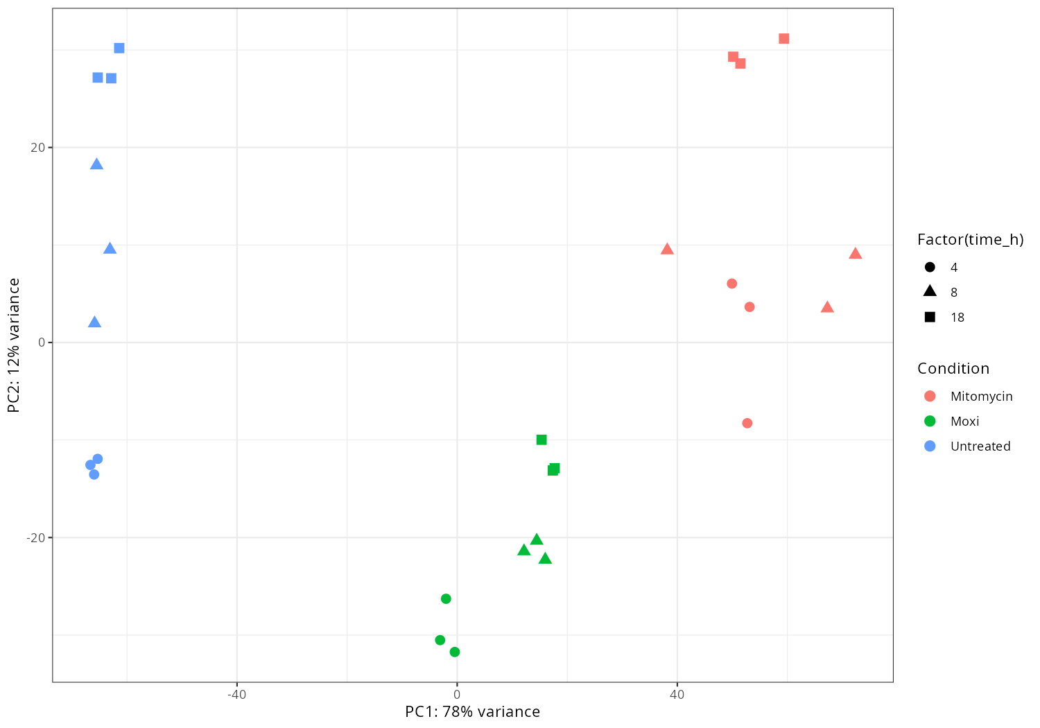
 png("pca2.png", 1200, 800)
 plotPCA(rld, intgroup=c("condition"))
 dev.off()

 png("pca3.png", 1200, 800)
 plotPCA(rld, intgroup=c("replicate"))
 dev.off()

 pdat <- plotPCA(rld, intgroup = c("condition","replicate"), returnData = TRUE)
 percentVar <- round(100 * attr(pdat, "percentVar"))
 # 1) keep only non-WT samples
 #pdat <- subset(pdat, !grepl("^WT_", condition))
 # drop unused factor levels so empty WT facets disappear
 pdat$condition <- droplevels(pdat$condition)
 # 2) pretty condition names: deltaadeIJ -> ΔadeIJ
 pdat$condition <- gsub("^deltaadeIJ", "\u0394adeIJ", pdat$condition)
 png("pca4.png", 1200, 800)
 ggplot(pdat, aes(PC1, PC2, color = replicate)) +
   geom_point(size = 3) +
   facet_wrap(~ condition) +
   xlab(paste0("PC1: ", percentVar[1], "% variance")) +
   ylab(paste0("PC2: ", percentVar[2], "% variance")) +
   theme_classic()
 dev.off()

 pdat <- plotPCA(rld, intgroup = c("condition","replicate"), returnData = TRUE)
 percentVar <- round(100 * attr(pdat, "percentVar"))
 # Drop WT_* conditions from the data and from factor levels
 pdat <- subset(pdat, !grepl("^WT_", condition))
 pdat$condition <- droplevels(pdat$condition)
 # Prettify condition labels for the legend: deltaadeIJ -> ΔadeIJ
 pdat$condition <- gsub("^deltaadeIJ", "\u0394adeIJ", pdat$condition)
 p <- ggplot(pdat, aes(PC1, PC2, color = replicate, shape = condition)) +
   geom_point(size = 3) +
   xlab(paste0("PC1: ", percentVar[1], "% variance")) +
   ylab(paste0("PC2: ", percentVar[2], "% variance")) +
   theme_classic()
 png("pca5.png", 1200, 800); print(p); dev.off()

 pdat <- plotPCA(rld, intgroup = c("condition","replicate"), returnData = TRUE)
 percentVar <- round(100 * attr(pdat, "percentVar"))
 p_fac <- ggplot(pdat, aes(PC1, PC2, color = replicate)) +
   geom_point(size = 3) +
   facet_wrap(~ condition) +
   xlab(paste0("PC1: ", percentVar[1], "% variance")) +
   ylab(paste0("PC2: ", percentVar[2], "% variance")) +
   theme_classic()
 png("pca6.png", 1200, 800); print(p_fac); dev.off()

 # -- heatmap --
 png("heatmap2.png", 1200, 800)
 distsRL <- dist(t(assay(rld)))
 mat <- as.matrix(distsRL)
 hc <- hclust(distsRL)
 hmcol <- colorRampPalette(brewer.pal(9,"GnBu"))(100)
 heatmap.2(mat, Rowv=as.dendrogram(hc),symm=TRUE, trace="none",col = rev(hmcol), margin=c(13, 13))
 dev.off()

 # -- pca_media_strain --
 #png("pca_media.png", 1200, 800)
 #plotPCA(rld, intgroup=c("media"))
 #dev.off()
 #png("pca_strain.png", 1200, 800)
 #plotPCA(rld, intgroup=c("strain"))
 #dev.off()
 #png("pca_time.png", 1200, 800)
 #plotPCA(rld, intgroup=c("time"))
 #dev.off()
-
Select the differentially expressed genes
 #https://galaxyproject.eu/posts/2020/08/22/three-steps-to-galaxify-your-tool/
 #https://www.biostars.org/p/282295/
 #https://www.biostars.org/p/335751/
 dds$condition
 [1] WT_none_17         WT_none_17         WT_none_17         WT_none_24
 [5] WT_none_24         WT_none_24         deltaadeIJ_none_17 deltaadeIJ_none_17
 [9] deltaadeIJ_none_17 deltaadeIJ_none_24 deltaadeIJ_none_24 deltaadeIJ_none_24
 [13] WT_one_17          WT_one_17          WT_one_17          WT_one_24
 [17] WT_one_24          WT_one_24          deltaadeIJ_one_17  deltaadeIJ_one_17
 [21] deltaadeIJ_one_17  deltaadeIJ_one_24  deltaadeIJ_one_24  deltaadeIJ_one_24
 [25] WT_two_17          WT_two_17          WT_two_17          WT_two_24
 [29] WT_two_24          WT_two_24          deltaadeIJ_two_17  deltaadeIJ_two_17
 [33] deltaadeIJ_two_17  deltaadeIJ_two_24  deltaadeIJ_two_24  deltaadeIJ_two_24
 12 Levels: deltaadeIJ_none_17 deltaadeIJ_none_24 ... WT_two_24

 #CONSOLE: mkdir star_salmon/degenes

 setwd("degenes")

 # Construct colData automatically
 sample_table <- data.frame(
     condition = condition,
     replicate = replicate
 )
 split_cond <- do.call(rbind, strsplit(as.character(condition), "_"))
 colnames(split_cond) <- c("genotype", "exposure", "time")
 colData <- cbind(sample_table, split_cond)
 colData$genotype <- factor(colData$genotype)
 colData$exposure  <- factor(colData$exposure)
 colData$time   <- factor(colData$time)
 colData$group  <- factor(paste(colData$genotype, colData$exposure, colData$time, sep = "_"))
 # Construct colData manually
 colData2 <- data.frame(condition=condition, row.names=names(files))

 # 确保因子顺序(可选)
 colData$genotype <- relevel(factor(colData$genotype), ref = "WT")
 colData$exposure  <- relevel(factor(colData$exposure), ref = "none")
 colData$time   <- relevel(factor(colData$time), ref = "17")

 dds <- DESeqDataSetFromTximport(txi, colData, design = ~ genotype * exposure * time)
 dds <- DESeq(dds, betaPrior = FALSE)
 resultsNames(dds)
 [1] "Intercept"
 [2] "genotype_deltaadeIJ_vs_WT"
 [3] "exposure_one_vs_none"
 [4] "exposure_two_vs_none"
 [5] "time_24_vs_17"
 [6] "genotypedeltaadeIJ.exposureone"
 [7] "genotypedeltaadeIJ.exposuretwo"
 [8] "genotypedeltaadeIJ.time24"
 [9] "exposureone.time24"
 [10] "exposuretwo.time24"
 [11] "genotypedeltaadeIJ.exposureone.time24"
 [12] "genotypedeltaadeIJ.exposuretwo.time24"

 # 提取 genotype 的主效应: up 10, down 4
 contrast <- "genotype_deltaadeIJ_vs_WT"
 res = results(dds, name=contrast)
 res <- res[!is.na(res$log2FoldChange),]
 res_df <- as.data.frame(res)
 write.csv(as.data.frame(res_df[order(res_df$pvalue),]), file = paste(contrast, "all.txt", sep="-"))
 up <- subset(res_df, padj<=0.05 & log2FoldChange>=2)
 down <- subset(res_df, padj<=0.05 & log2FoldChange<=-2)
 write.csv(as.data.frame(up[order(up$log2FoldChange,decreasing=TRUE),]), file = paste(contrast, "up.txt", sep="-"))
 write.csv(as.data.frame(down[order(abs(down$log2FoldChange),decreasing=TRUE),]), file = paste(contrast, "down.txt", sep="-"))

 # 提取 one exposure 的主效应: up 196; down 298
 contrast <- "exposure_one_vs_none"
 res = results(dds, name=contrast)
 res <- res[!is.na(res$log2FoldChange),]
 res_df <- as.data.frame(res)
 write.csv(as.data.frame(res_df[order(res_df$pvalue),]), file = paste(contrast, "all.txt", sep="-"))
 up <- subset(res_df, padj<=0.05 & log2FoldChange>=2)
 down <- subset(res_df, padj<=0.05 & log2FoldChange<=-2)
 write.csv(as.data.frame(up[order(up$log2FoldChange,decreasing=TRUE),]), file = paste(contrast, "up.txt", sep="-"))
 write.csv(as.data.frame(down[order(abs(down$log2FoldChange),decreasing=TRUE),]), file = paste(contrast, "down.txt", sep="-"))

 # 提取 two exposure 的主效应: up 80; down 105
 contrast <- "exposure_two_vs_none"
 res = results(dds, name=contrast)
 res <- res[!is.na(res$log2FoldChange),]
 res_df <- as.data.frame(res)
 write.csv(as.data.frame(res_df[order(res_df$pvalue),]), file = paste(contrast, "all.txt", sep="-"))
 up <- subset(res_df, padj<=0.05 & log2FoldChange>=2)
 down <- subset(res_df, padj<=0.05 & log2FoldChange<=-2)
 write.csv(as.data.frame(up[order(up$log2FoldChange,decreasing=TRUE),]), file = paste(contrast, "up.txt", sep="-"))
 write.csv(as.data.frame(down[order(abs(down$log2FoldChange),decreasing=TRUE),]), file = paste(contrast, "down.txt", sep="-"))

 # 提取 time 的主效应 up 10; down 2
 contrast <- "time_24_vs_17"
 res = results(dds, name=contrast)
 res <- res[!is.na(res$log2FoldChange),]
 res_df <- as.data.frame(res)
 write.csv(as.data.frame(res_df[order(res_df$pvalue),]), file = paste(contrast, "all.txt", sep="-"))
 up <- subset(res_df, padj<=0.05 & log2FoldChange>=2)
 down <- subset(res_df, padj<=0.05 & log2FoldChange<=-2)
 write.csv(as.data.frame(up[order(up$log2FoldChange,decreasing=TRUE),]), file = paste(contrast, "up.txt", sep="-"))
 write.csv(as.data.frame(down[order(abs(down$log2FoldChange),decreasing=TRUE),]), file = paste(contrast, "down.txt", sep="-"))

 #1.)  ΔadeIJ_none 17h vs WT_none 17h
 #2.)  ΔadeIJ_none 24h vs WT_none 24h
 #3.)  ΔadeIJ_one 17h vs WT_one 17h
 #4.)  ΔadeIJ_one 24h vs WT_one 24h
 #5.)  ΔadeIJ_two 17h vs WT_two 17h
 #6.)  ΔadeIJ_two 24h vs WT_two 24h

 #---- relevel to control ----
 dds <- DESeqDataSetFromTximport(txi, colData, design = ~ condition)
 dds$condition <- relevel(dds$condition, "WT_none_17")
 dds = DESeq(dds, betaPrior=FALSE)
 resultsNames(dds)
 clist <- c("deltaadeIJ_none_17_vs_WT_none_17")

 dds$condition <- relevel(dds$condition, "WT_none_24")
 dds = DESeq(dds, betaPrior=FALSE)
 resultsNames(dds)
 clist <- c("deltaadeIJ_none_24_vs_WT_none_24")

 dds$condition <- relevel(dds$condition, "WT_one_17")
 dds = DESeq(dds, betaPrior=FALSE)
 resultsNames(dds)
 clist <- c("deltaadeIJ_one_17_vs_WT_one_17")

 dds$condition <- relevel(dds$condition, "WT_one_24")
 dds = DESeq(dds, betaPrior=FALSE)
 resultsNames(dds)
 clist <- c("deltaadeIJ_one_24_vs_WT_one_24")

 dds$condition <- relevel(dds$condition, "WT_two_17")
 dds = DESeq(dds, betaPrior=FALSE)
 resultsNames(dds)
 clist <- c("deltaadeIJ_two_17_vs_WT_two_17")

 dds$condition <- relevel(dds$condition, "WT_two_24")
 dds = DESeq(dds, betaPrior=FALSE)
 resultsNames(dds)
 clist <- c("deltaadeIJ_two_24_vs_WT_two_24")

 # WT_none_xh
 dds$condition <- relevel(dds$condition, "WT_none_17")
 dds = DESeq(dds, betaPrior=FALSE)
 resultsNames(dds)
 clist <- c("WT_none_24_vs_WT_none_17")

 # WT_one_xh
 dds$condition <- relevel(dds$condition, "WT_one_17")
 dds = DESeq(dds, betaPrior=FALSE)
 resultsNames(dds)
 clist <- c("WT_one_24_vs_WT_one_17")

 # WT_two_xh
 dds$condition <- relevel(dds$condition, "WT_two_17")
 dds = DESeq(dds, betaPrior=FALSE)
 resultsNames(dds)
 clist <- c("WT_two_24_vs_WT_two_17")

 # deltaadeIJ_none_xh
 dds$condition <- relevel(dds$condition, "deltaadeIJ_none_17")
 dds = DESeq(dds, betaPrior=FALSE)
 resultsNames(dds)
 clist <- c("deltaadeIJ_none_24_vs_deltaadeIJ_none_17")

 # deltaadeIJ_one_xh
 dds$condition <- relevel(dds$condition, "deltaadeIJ_one_17")
 dds = DESeq(dds, betaPrior=FALSE)
 resultsNames(dds)
 clist <- c("deltaadeIJ_one_24_vs_deltaadeIJ_one_17")

 # deltaadeIJ_two_xh
 dds$condition <- relevel(dds$condition, "deltaadeIJ_two_17")
 dds = DESeq(dds, betaPrior=FALSE)
 resultsNames(dds)
 clist <- c("deltaadeIJ_two_24_vs_deltaadeIJ_two_17")

 for (i in clist) {
   contrast = paste("condition", i, sep="_")
   #for_Mac_vs_LB  contrast = paste("media", i, sep="_")
   res = results(dds, name=contrast)
   res <- res[!is.na(res$log2FoldChange),]
   res_df <- as.data.frame(res)

   write.csv(as.data.frame(res_df[order(res_df$pvalue),]), file = paste(i, "all.txt", sep="-"))
   #res$log2FoldChange < -2 & res$padj < 5e-2
   up <- subset(res_df, padj<=0.05 & log2FoldChange>=2)
   down <- subset(res_df, padj<=0.05 & log2FoldChange<=-2)
   write.csv(as.data.frame(up[order(up$log2FoldChange,decreasing=TRUE),]), file = paste(i, "up.txt", sep="-"))
   write.csv(as.data.frame(down[order(abs(down$log2FoldChange),decreasing=TRUE),]), file = paste(i, "down.txt", sep="-"))
 }

 # -- Under host-env (mamba activate plot-numpy1) --
 mamba activate plot-numpy1
 grep -P "\tgene\t" CP059040_m.gff > CP059040_gene.gff

 for cmp in deltaadeIJ_none_17_vs_WT_none_17 deltaadeIJ_none_24_vs_WT_none_24 deltaadeIJ_one_17_vs_WT_one_17 deltaadeIJ_one_24_vs_WT_one_24 deltaadeIJ_two_17_vs_WT_two_17 deltaadeIJ_two_24_vs_WT_two_24    WT_none_24_vs_WT_none_17 WT_one_24_vs_WT_one_17 WT_two_24_vs_WT_two_17 deltaadeIJ_none_24_vs_deltaadeIJ_none_17 deltaadeIJ_one_24_vs_deltaadeIJ_one_17 deltaadeIJ_two_24_vs_deltaadeIJ_two_17; do
   python3 ~/Scripts/replace_gene_names.py /home/jhuang/DATA/Data_Tam_RNAseq_2025_subMIC_exposure_ATCC19606/CP059040_gene.gff ${cmp}-all.txt ${cmp}-all.csv
   python3 ~/Scripts/replace_gene_names.py /home/jhuang/DATA/Data_Tam_RNAseq_2025_subMIC_exposure_ATCC19606/CP059040_gene.gff ${cmp}-up.txt ${cmp}-up.csv
   python3 ~/Scripts/replace_gene_names.py /home/jhuang/DATA/Data_Tam_RNAseq_2025_subMIC_exposure_ATCC19606/CP059040_gene.gff ${cmp}-down.txt ${cmp}-down.csv
 done
 #deltaadeIJ_none_24_vs_deltaadeIJ_none_17  up(0) down(0)
 #deltaadeIJ_one_24_vs_deltaadeIJ_one_17    up(0) down(8: gabT, H0N29_11475, H0N29_01015, H0N29_01030, ...)
 #deltaadeIJ_two_24_vs_deltaadeIJ_two_17    up(8) down(51)
-
(NOT_PERFORMED) Volcano plots
 # ---- delta sbp TSB 2h vs WT TSB 2h ----
 res <- read.csv("deltasbp_TSB_2h_vs_WT_TSB_2h-all.csv")
 # Replace empty GeneName with modified GeneID
 res$GeneName <- ifelse(
   res$GeneName == "" | is.na(res$GeneName),
   gsub("gene-", "", res$GeneID),
   res$GeneName
 )
 duplicated_genes <- res[duplicated(res$GeneName), "GeneName"]
 #print(duplicated_genes)
 # [1] "bfr"  "lipA" "ahpF" "pcaF" "alr"  "pcaD" "cydB" "lpdA" "pgaC" "ppk1"
 #[11] "pcaF" "tuf"  "galE" "murI" "yccS" "rrf"  "rrf"  "arsB" "ptsP" "umuD"
 #[21] "map"  "pgaB" "rrf"  "rrf"  "rrf"  "pgaD" "uraH" "benE"
 #res[res$GeneName == "bfr", ]

 #1st_strategy First occurrence is kept and Subsequent duplicates are removed
 #res <- res[!duplicated(res$GeneName), ]
 #2nd_strategy keep the row with the smallest padj value for each GeneName
 res <- res %>%
   group_by(GeneName) %>%
   slice_min(padj, with_ties = FALSE) %>%
   ungroup()
 res <- as.data.frame(res)
 # Sort res first by padj (ascending) and then by log2FoldChange (descending)
 res <- res[order(res$padj, -res$log2FoldChange), ]

 # Assuming res is your dataframe and already processed
 # Filter up-regulated genes: log2FoldChange > 2 and padj < 5e-2
 up_regulated <- res[res$log2FoldChange > 2 & res$padj < 5e-2, ]
 # Filter down-regulated genes: log2FoldChange < -2 and padj < 5e-2
 down_regulated <- res[res$log2FoldChange < -2 & res$padj < 5e-2, ]
 # Create a new workbook
 wb <- createWorkbook()
 # Add the complete dataset as the first sheet
 addWorksheet(wb, "Complete_Data")
 writeData(wb, "Complete_Data", res)
 # Add the up-regulated genes as the second sheet
 addWorksheet(wb, "Up_Regulated")
 writeData(wb, "Up_Regulated", up_regulated)
 # Add the down-regulated genes as the third sheet
 addWorksheet(wb, "Down_Regulated")
 writeData(wb, "Down_Regulated", down_regulated)
 # Save the workbook to a file
 saveWorkbook(wb, "Gene_Expression_Δsbp_TSB_2h_vs_WT_TSB_2h.xlsx", overwrite = TRUE)

 # Set the 'GeneName' column as row.names
 rownames(res) <- res$GeneName
 # Drop the 'GeneName' column since it's now the row names
 res$GeneName <- NULL
 head(res)

 ## Ensure the data frame matches the expected format
 ## For example, it should have columns: log2FoldChange, padj, etc.
 #res <- as.data.frame(res)
 ## Remove rows with NA in log2FoldChange (if needed)
 #res <- res[!is.na(res$log2FoldChange),]

 # Replace padj = 0 with a small value
 #NO_SUCH_RECORDS: res$padj[res$padj == 0] <- 1e-150

 #library(EnhancedVolcano)
 # Assuming res is already sorted and processed
 png("Δsbp_TSB_2h_vs_WT_TSB_2h.png", width=1200, height=1200)
 #max.overlaps = 10
 EnhancedVolcano(res,
                 lab = rownames(res),
                 x = 'log2FoldChange',
                 y = 'padj',
                 pCutoff = 5e-2,
                 FCcutoff = 2,
                 title = '',
                 subtitleLabSize = 18,
                 pointSize = 3.0,
                 labSize = 5.0,
                 colAlpha = 1,
                 legendIconSize = 4.0,
                 drawConnectors = TRUE,
                 widthConnectors = 0.5,
                 colConnectors = 'black',
                 subtitle = expression("Δsbp TSB 2h versus WT TSB 2h"))
 dev.off()

 # ---- delta sbp TSB 4h vs WT TSB 4h ----
 res <- read.csv("deltasbp_TSB_4h_vs_WT_TSB_4h-all.csv")
 # Replace empty GeneName with modified GeneID
 res$GeneName <- ifelse(
   res$GeneName == "" | is.na(res$GeneName),
   gsub("gene-", "", res$GeneID),
   res$GeneName
 )
 duplicated_genes <- res[duplicated(res$GeneName), "GeneName"]

 res <- res %>%
   group_by(GeneName) %>%
   slice_min(padj, with_ties = FALSE) %>%
   ungroup()
 res <- as.data.frame(res)
 # Sort res first by padj (ascending) and then by log2FoldChange (descending)
 res <- res[order(res$padj, -res$log2FoldChange), ]

 # Assuming res is your dataframe and already processed
 # Filter up-regulated genes: log2FoldChange > 2 and padj < 5e-2
 up_regulated <- res[res$log2FoldChange > 2 & res$padj < 5e-2, ]
 # Filter down-regulated genes: log2FoldChange < -2 and padj < 5e-2
 down_regulated <- res[res$log2FoldChange < -2 & res$padj < 5e-2, ]
 # Create a new workbook
 wb <- createWorkbook()
 # Add the complete dataset as the first sheet
 addWorksheet(wb, "Complete_Data")
 writeData(wb, "Complete_Data", res)
 # Add the up-regulated genes as the second sheet
 addWorksheet(wb, "Up_Regulated")
 writeData(wb, "Up_Regulated", up_regulated)
 # Add the down-regulated genes as the third sheet
 addWorksheet(wb, "Down_Regulated")
 writeData(wb, "Down_Regulated", down_regulated)
 # Save the workbook to a file
 saveWorkbook(wb, "Gene_Expression_Δsbp_TSB_4h_vs_WT_TSB_4h.xlsx", overwrite = TRUE)

 # Set the 'GeneName' column as row.names
 rownames(res) <- res$GeneName
 # Drop the 'GeneName' column since it's now the row names
 res$GeneName <- NULL
 head(res)

 #library(EnhancedVolcano)
 # Assuming res is already sorted and processed
 png("Δsbp_TSB_4h_vs_WT_TSB_4h.png", width=1200, height=1200)
 #max.overlaps = 10
 EnhancedVolcano(res,
                 lab = rownames(res),
                 x = 'log2FoldChange',
                 y = 'padj',
                 pCutoff = 5e-2,
                 FCcutoff = 2,
                 title = '',
                 subtitleLabSize = 18,
                 pointSize = 3.0,
                 labSize = 5.0,
                 colAlpha = 1,
                 legendIconSize = 4.0,
                 drawConnectors = TRUE,
                 widthConnectors = 0.5,
                 colConnectors = 'black',
                 subtitle = expression("Δsbp TSB 4h versus WT TSB 4h"))
 dev.off()

 # ---- delta sbp TSB 18h vs WT TSB 18h ----
 res <- read.csv("deltasbp_TSB_18h_vs_WT_TSB_18h-all.csv")
 # Replace empty GeneName with modified GeneID
 res$GeneName <- ifelse(
   res$GeneName == "" | is.na(res$GeneName),
   gsub("gene-", "", res$GeneID),
   res$GeneName
 )
 duplicated_genes <- res[duplicated(res$GeneName), "GeneName"]

 res <- res %>%
   group_by(GeneName) %>%
   slice_min(padj, with_ties = FALSE) %>%
   ungroup()
 res <- as.data.frame(res)
 # Sort res first by padj (ascending) and then by log2FoldChange (descending)
 res <- res[order(res$padj, -res$log2FoldChange), ]

 # Assuming res is your dataframe and already processed
 # Filter up-regulated genes: log2FoldChange > 2 and padj < 5e-2
 up_regulated <- res[res$log2FoldChange > 2 & res$padj < 5e-2, ]
 # Filter down-regulated genes: log2FoldChange < -2 and padj < 5e-2
 down_regulated <- res[res$log2FoldChange < -2 & res$padj < 5e-2, ]
 # Create a new workbook
 wb <- createWorkbook()
 # Add the complete dataset as the first sheet
 addWorksheet(wb, "Complete_Data")
 writeData(wb, "Complete_Data", res)
 # Add the up-regulated genes as the second sheet
 addWorksheet(wb, "Up_Regulated")
 writeData(wb, "Up_Regulated", up_regulated)
 # Add the down-regulated genes as the third sheet
 addWorksheet(wb, "Down_Regulated")
 writeData(wb, "Down_Regulated", down_regulated)
 # Save the workbook to a file
 saveWorkbook(wb, "Gene_Expression_Δsbp_TSB_18h_vs_WT_TSB_18h.xlsx", overwrite = TRUE)

 # Set the 'GeneName' column as row.names
 rownames(res) <- res$GeneName
 # Drop the 'GeneName' column since it's now the row names
 res$GeneName <- NULL
 head(res)

 #library(EnhancedVolcano)
 # Assuming res is already sorted and processed
 png("Δsbp_TSB_18h_vs_WT_TSB_18h.png", width=1200, height=1200)
 #max.overlaps = 10
 EnhancedVolcano(res,
                 lab = rownames(res),
                 x = 'log2FoldChange',
                 y = 'padj',
                 pCutoff = 5e-2,
                 FCcutoff = 2,
                 title = '',
                 subtitleLabSize = 18,
                 pointSize = 3.0,
                 labSize = 5.0,
                 colAlpha = 1,
                 legendIconSize = 4.0,
                 drawConnectors = TRUE,
                 widthConnectors = 0.5,
                 colConnectors = 'black',
                 subtitle = expression("Δsbp TSB 18h versus WT TSB 18h"))
 dev.off()

 # ---- delta sbp MH 2h vs WT MH 2h ----
 res <- read.csv("deltasbp_MH_2h_vs_WT_MH_2h-all.csv")
 # Replace empty GeneName with modified GeneID
 res$GeneName <- ifelse(
   res$GeneName == "" | is.na(res$GeneName),
   gsub("gene-", "", res$GeneID),
   res$GeneName
 )
 duplicated_genes <- res[duplicated(res$GeneName), "GeneName"]
 #print(duplicated_genes)
 # [1] "bfr"  "lipA" "ahpF" "pcaF" "alr"  "pcaD" "cydB" "lpdA" "pgaC" "ppk1"
 #[11] "pcaF" "tuf"  "galE" "murI" "yccS" "rrf"  "rrf"  "arsB" "ptsP" "umuD"
 #[21] "map"  "pgaB" "rrf"  "rrf"  "rrf"  "pgaD" "uraH" "benE"
 #res[res$GeneName == "bfr", ]

 #1st_strategy First occurrence is kept and Subsequent duplicates are removed
 #res <- res[!duplicated(res$GeneName), ]
 #2nd_strategy keep the row with the smallest padj value for each GeneName
 res <- res %>%
   group_by(GeneName) %>%
   slice_min(padj, with_ties = FALSE) %>%
   ungroup()
 res <- as.data.frame(res)
 # Sort res first by padj (ascending) and then by log2FoldChange (descending)
 res <- res[order(res$padj, -res$log2FoldChange), ]

 # Assuming res is your dataframe and already processed
 # Filter up-regulated genes: log2FoldChange > 2 and padj < 5e-2
 up_regulated <- res[res$log2FoldChange > 2 & res$padj < 5e-2, ]
 # Filter down-regulated genes: log2FoldChange < -2 and padj < 5e-2
 down_regulated <- res[res$log2FoldChange < -2 & res$padj < 5e-2, ]
 # Create a new workbook
 wb <- createWorkbook()
 # Add the complete dataset as the first sheet
 addWorksheet(wb, "Complete_Data")
 writeData(wb, "Complete_Data", res)
 # Add the up-regulated genes as the second sheet
 addWorksheet(wb, "Up_Regulated")
 writeData(wb, "Up_Regulated", up_regulated)
 # Add the down-regulated genes as the third sheet
 addWorksheet(wb, "Down_Regulated")
 writeData(wb, "Down_Regulated", down_regulated)
 # Save the workbook to a file
 saveWorkbook(wb, "Gene_Expression_Δsbp_MH_2h_vs_WT_MH_2h.xlsx", overwrite = TRUE)

 # Set the 'GeneName' column as row.names
 rownames(res) <- res$GeneName
 # Drop the 'GeneName' column since it's now the row names
 res$GeneName <- NULL
 head(res)

 ## Ensure the data frame matches the expected format
 ## For example, it should have columns: log2FoldChange, padj, etc.
 #res <- as.data.frame(res)
 ## Remove rows with NA in log2FoldChange (if needed)
 #res <- res[!is.na(res$log2FoldChange),]

 # Replace padj = 0 with a small value
 #NO_SUCH_RECORDS: res$padj[res$padj == 0] <- 1e-150

 #library(EnhancedVolcano)
 # Assuming res is already sorted and processed
 png("Δsbp_MH_2h_vs_WT_MH_2h.png", width=1200, height=1200)
 #max.overlaps = 10
 EnhancedVolcano(res,
                 lab = rownames(res),
                 x = 'log2FoldChange',
                 y = 'padj',
                 pCutoff = 5e-2,
                 FCcutoff = 2,
                 title = '',
                 subtitleLabSize = 18,
                 pointSize = 3.0,
                 labSize = 5.0,
                 colAlpha = 1,
                 legendIconSize = 4.0,
                 drawConnectors = TRUE,
                 widthConnectors = 0.5,
                 colConnectors = 'black',
                 subtitle = expression("Δsbp MH 2h versus WT MH 2h"))
 dev.off()

 # ---- delta sbp MH 4h vs WT MH 4h ----
 res <- read.csv("deltasbp_MH_4h_vs_WT_MH_4h-all.csv")
 # Replace empty GeneName with modified GeneID
 res$GeneName <- ifelse(
   res$GeneName == "" | is.na(res$GeneName),
   gsub("gene-", "", res$GeneID),
   res$GeneName
 )
 duplicated_genes <- res[duplicated(res$GeneName), "GeneName"]

 res <- res %>%
   group_by(GeneName) %>%
   slice_min(padj, with_ties = FALSE) %>%
   ungroup()
 res <- as.data.frame(res)
 # Sort res first by padj (ascending) and then by log2FoldChange (descending)
 res <- res[order(res$padj, -res$log2FoldChange), ]

 # Assuming res is your dataframe and already processed
 # Filter up-regulated genes: log2FoldChange > 2 and padj < 5e-2
 up_regulated <- res[res$log2FoldChange > 2 & res$padj < 5e-2, ]
 # Filter down-regulated genes: log2FoldChange < -2 and padj < 5e-2
 down_regulated <- res[res$log2FoldChange < -2 & res$padj < 5e-2, ]
 # Create a new workbook
 wb <- createWorkbook()
 # Add the complete dataset as the first sheet
 addWorksheet(wb, "Complete_Data")
 writeData(wb, "Complete_Data", res)
 # Add the up-regulated genes as the second sheet
 addWorksheet(wb, "Up_Regulated")
 writeData(wb, "Up_Regulated", up_regulated)
 # Add the down-regulated genes as the third sheet
 addWorksheet(wb, "Down_Regulated")
 writeData(wb, "Down_Regulated", down_regulated)
 # Save the workbook to a file
 saveWorkbook(wb, "Gene_Expression_Δsbp_MH_4h_vs_WT_MH_4h.xlsx", overwrite = TRUE)

 # Set the 'GeneName' column as row.names
 rownames(res) <- res$GeneName
 # Drop the 'GeneName' column since it's now the row names
 res$GeneName <- NULL
 head(res)

 #library(EnhancedVolcano)
 # Assuming res is already sorted and processed
 png("Δsbp_MH_4h_vs_WT_MH_4h.png", width=1200, height=1200)
 #max.overlaps = 10
 EnhancedVolcano(res,
                 lab = rownames(res),
                 x = 'log2FoldChange',
                 y = 'padj',
                 pCutoff = 5e-2,
                 FCcutoff = 2,
                 title = '',
                 subtitleLabSize = 18,
                 pointSize = 3.0,
                 labSize = 5.0,
                 colAlpha = 1,
                 legendIconSize = 4.0,
                 drawConnectors = TRUE,
                 widthConnectors = 0.5,
                 colConnectors = 'black',
                 subtitle = expression("Δsbp MH 4h versus WT MH 4h"))
 dev.off()

 # ---- delta sbp MH 18h vs WT MH 18h ----
 res <- read.csv("deltasbp_MH_18h_vs_WT_MH_18h-all.csv")
 # Replace empty GeneName with modified GeneID
 res$GeneName <- ifelse(
   res$GeneName == "" | is.na(res$GeneName),
   gsub("gene-", "", res$GeneID),
   res$GeneName
 )
 duplicated_genes <- res[duplicated(res$GeneName), "GeneName"]

 res <- res %>%
   group_by(GeneName) %>%
   slice_min(padj, with_ties = FALSE) %>%
   ungroup()
 res <- as.data.frame(res)
 # Sort res first by padj (ascending) and then by log2FoldChange (descending)
 res <- res[order(res$padj, -res$log2FoldChange), ]

 # Assuming res is your dataframe and already processed
 # Filter up-regulated genes: log2FoldChange > 2 and padj < 5e-2
 up_regulated <- res[res$log2FoldChange > 2 & res$padj < 5e-2, ]
 # Filter down-regulated genes: log2FoldChange < -2 and padj < 5e-2
 down_regulated <- res[res$log2FoldChange < -2 & res$padj < 5e-2, ]
 # Create a new workbook
 wb <- createWorkbook()
 # Add the complete dataset as the first sheet
 addWorksheet(wb, "Complete_Data")
 writeData(wb, "Complete_Data", res)
 # Add the up-regulated genes as the second sheet
 addWorksheet(wb, "Up_Regulated")
 writeData(wb, "Up_Regulated", up_regulated)
 # Add the down-regulated genes as the third sheet
 addWorksheet(wb, "Down_Regulated")
 writeData(wb, "Down_Regulated", down_regulated)
 # Save the workbook to a file
 saveWorkbook(wb, "Gene_Expression_Δsbp_MH_18h_vs_WT_MH_18h.xlsx", overwrite = TRUE)

 # Set the 'GeneName' column as row.names
 rownames(res) <- res$GeneName
 # Drop the 'GeneName' column since it's now the row names
 res$GeneName <- NULL
 head(res)

 #library(EnhancedVolcano)
 # Assuming res is already sorted and processed
 png("Δsbp_MH_18h_vs_WT_MH_18h.png", width=1200, height=1200)
 #max.overlaps = 10
 EnhancedVolcano(res,
                 lab = rownames(res),
                 x = 'log2FoldChange',
                 y = 'padj',
                 pCutoff = 5e-2,
                 FCcutoff = 2,
                 title = '',
                 subtitleLabSize = 18,
                 pointSize = 3.0,
                 labSize = 5.0,
                 colAlpha = 1,
                 legendIconSize = 4.0,
                 drawConnectors = TRUE,
                 widthConnectors = 0.5,
                 colConnectors = 'black',
                 subtitle = expression("Δsbp MH 18h versus WT MH 18h"))
 dev.off()

 #Annotate the Gene_Expression_xxx_vs_yyy.xlsx in the next steps (see below e.g. Gene_Expression_with_Annotations_Urine_vs_MHB.xlsx)
KEGG and GO annotations in non-model organisms
https://www.biobam.com/functional-analysis/
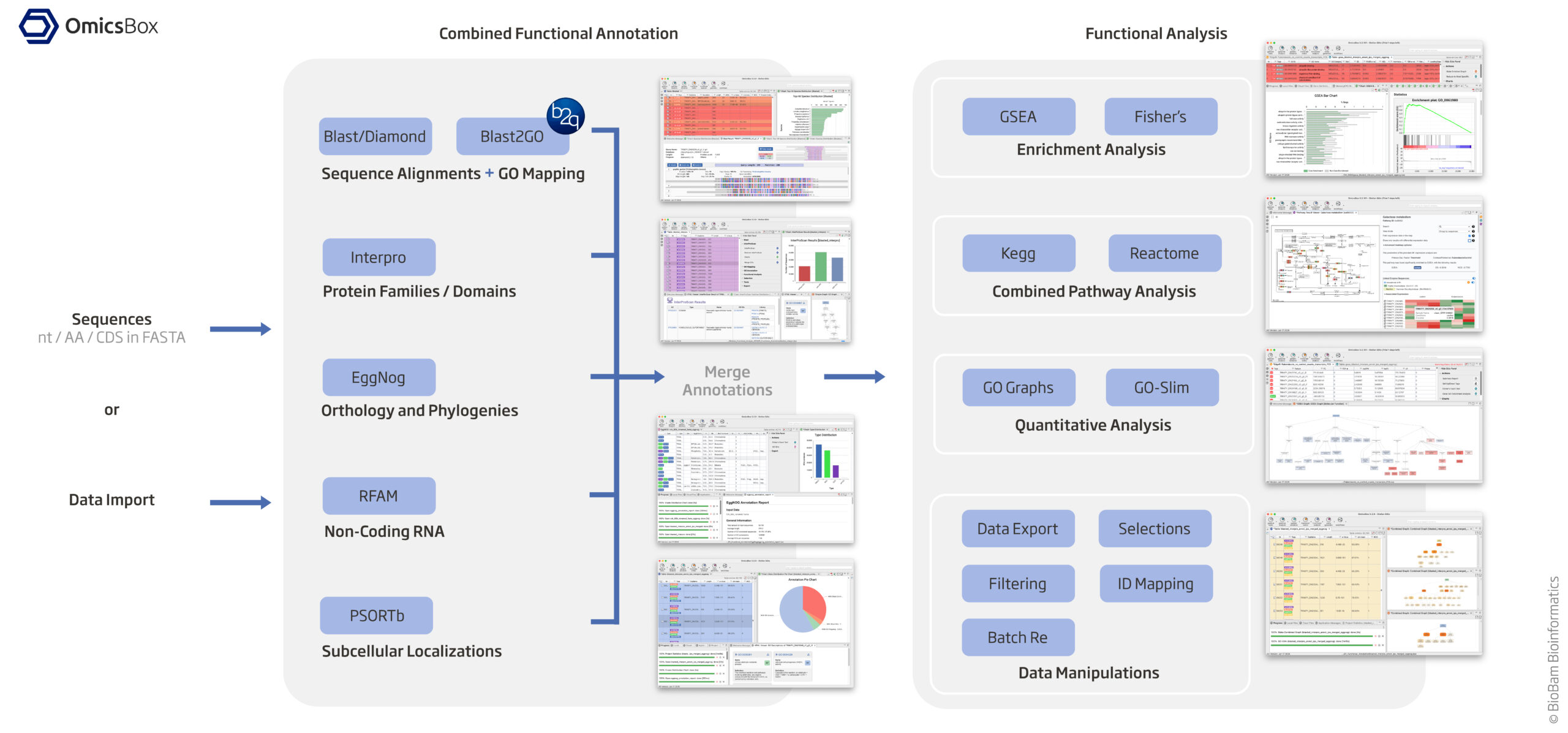
10.1. Assign KEGG and GO Terms (see diagram above)
    Since your organism is non-model, standard R databases (org.Hs.eg.db, etc.) won’t work. You’ll need to manually retrieve KEGG and GO annotations.

    Option 1 (KEGG Terms): EggNog based on orthology and phylogenies

        EggNOG-mapper assigns both KEGG Orthology (KO) IDs and GO terms.

        Install EggNOG-mapper:

            mamba create -n eggnog_env python=3.8 eggnog-mapper -c conda-forge -c bioconda  #eggnog-mapper_2.1.12
            mamba activate eggnog_env

        Run annotation:

            #diamond makedb --in eggnog6.prots.faa -d eggnog_proteins.dmnd
            mkdir /home/jhuang/mambaforge/envs/eggnog_env/lib/python3.8/site-packages/data/
            download_eggnog_data.py --dbname eggnog.db -y --data_dir /home/jhuang/mambaforge/envs/eggnog_env/lib/python3.8/site-packages/data/
            #NOT_WORKING: emapper.py -i CP020463_gene.fasta -o eggnog_dmnd_out --cpu 60 -m diamond[hmmer,mmseqs] --dmnd_db /home/jhuang/REFs/eggnog_data/data/eggnog_proteins.dmnd
            #Download the protein sequences from Genbank
            mv ~/Downloads/sequence\ \(3\).txt CP020463_protein_.fasta
            python ~/Scripts/update_fasta_header.py CP020463_protein_.fasta CP020463_protein.fasta
            emapper.py -i CP020463_protein.fasta -o eggnog_out --cpu 60  #--resume
            #----> result annotations.tsv: Contains KEGG, GO, and other functional annotations.
            #---->  470.IX87_14445:
                * 470 likely refers to the organism or strain (e.g., Acinetobacter baumannii ATCC 19606 or another related strain).
                * IX87_14445 would refer to a specific gene or protein within that genome.

        Extract KEGG KO IDs from annotations.emapper.annotations.

    Option 2 (GO Terms from 'Blast2GO 5 Basic', saved in blast2go_annot.annot): Using Blast/Diamond + Blast2GO_GUI based on sequence alignment + GO mapping

    * jhuang@WS-2290C:~/DATA/Data_Michelle_RNAseq_2025$ ~/Tools/Blast2GO/Blast2GO_Launcher setting the workspace "mkdir ~/b2gWorkspace_Michelle_RNAseq_2025"; cp /mnt/md1/DATA/Data_Michelle_RNAseq_2025/results/star_salmon/degenes/CP020463_protein.fasta ~/b2gWorkspace_Michelle_RNAseq_2025
    * 'Load protein sequences' (Tags: NONE, generated columns: Nr, SeqName) by choosing the file CP020463_protein.fasta as input -->
    * Buttons 'blast' at the NCBI (Parameters: blastp, nr, ...) (Tags: BLASTED, generated columns: Description, Length, #Hits, e-Value, sim mean),
            QBlast finished with warnings!
            Blasted Sequences: 2084
            Sequences without results: 105
            Check the Job log for details and try to submit again.
            Restarting QBlast may result in additional results, depending on the error type.
            "Blast (CP020463_protein) Done"
    * Button 'mapping' (Tags: MAPPED, generated columns: #GO, GO IDs, GO Names), "Mapping finished - Please proceed now to annotation."
            "Mapping (CP020463_protein) Done"
            "Mapping finished - Please proceed now to annotation."
    * Button 'annot' (Tags: ANNOTATED, generated columns: Enzyme Codes, Enzyme Names), "Annotation finished."
            * Used parameter 'Annotation CutOff': The Blast2GO Annotation Rule seeks to find the most specific GO annotations with a certain level of reliability. An annotation score is calculated for each candidate GO which is composed by the sequence similarity of the Blast Hit, the evidence code of the source GO and the position of the particular GO in the Gene Ontology hierarchy. This annotation score cutoff select the most specific GO term for a given GO branch which lies above this value.
            * Used parameter 'GO Weight' is a value which is added to Annotation Score of a more general/abstract Gene Ontology term for each of its more specific, original source GO terms. In this case, more general GO terms which summarise many original source terms (those ones directly associated to the Blast Hits) will have a higher Annotation Score.
            "Annotation (CP020463_protein) Done"
            "Annotation finished."
    or blast2go_cli_v1.5.1 (NOT_USED)

            #https://help.biobam.com/space/BCD/2250407989/Installation
            #see ~/Scripts/blast2go_pipeline.sh

    Option 3 (GO Terms from 'Blast2GO 5 Basic', saved in blast2go_annot.annot2): Interpro based protein families / domains --> Button interpro
        * Button 'interpro' (Tags: INTERPRO, generated columns: InterPro IDs, InterPro GO IDs, InterPro GO Names) --> "InterProScan Finished - You can now merge the obtained GO Annotations."
            "InterProScan (CP020463_protein) Done"
            "InterProScan Finished - You can now merge the obtained GO Annotations."
    MERGE the results of InterPro GO IDs (Option 3) to GO IDs (Option 2) and generate final GO IDs
        * Button 'interpro'/'Merge InterProScan GOs to Annotation' --> "Merge (add and validate) all GO terms retrieved via InterProScan to the already existing GO annotation."
            "Merge InterProScan GOs to Annotation (CP020463_protein) Done"
            "Finished merging GO terms from InterPro with annotations."
            "Maybe you want to run ANNEX (Annotation Augmentation)."
        #* Button 'annot'/'ANNEX' --> "ANNEX finished. Maybe you want to do the next step: Enzyme Code Mapping."
    File -> Export -> Export Annotations -> Export Annotations (.annot, custom, etc.)
            #~/b2gWorkspace_Michelle_RNAseq_2025/blast2go_annot.annot is generated!

        #-- before merging (blast2go_annot.annot) --
        #H0N29_18790     GO:0004842      ankyrin repeat domain-containing protein
        #H0N29_18790     GO:0085020
        #-- after merging (blast2go_annot.annot2) -->
        #H0N29_18790     GO:0031436      ankyrin repeat domain-containing protein
        #H0N29_18790     GO:0070531
        #H0N29_18790     GO:0004842
        #H0N29_18790     GO:0005515
        #H0N29_18790     GO:0085020

        cp blast2go_annot.annot blast2go_annot.annot2

    Option 4 (NOT_USED): RFAM for non-colding RNA

    Option 5 (NOT_USED): PSORTb for subcellular localizations

    Option 6 (NOT_USED): KAAS (KEGG Automatic Annotation Server)

    * Go to KAAS
    * Upload your FASTA file.
    * Select an appropriate gene set.
    * Download the KO assignments.
10.2. Find the Closest KEGG Organism Code (NOT_USED)
    Since your species isn't directly in KEGG, use a closely related organism.

    * Check available KEGG organisms:

            library(clusterProfiler)
            library(KEGGREST)

            kegg_organisms <- keggList("organism")

            Pick the closest relative (e.g., zebrafish "dre" for fish, Arabidopsis "ath" for plants).

            # Search for Acinetobacter in the list
            grep("Acinetobacter", kegg_organisms, ignore.case = TRUE, value = TRUE)
            # Gammaproteobacteria
            #Extract KO IDs from the eggnog results for  "Acinetobacter baumannii strain ATCC 19606"
10.3. Find the Closest KEGG Organism for a Non-Model Species (NOT_USED)
    If your organism is not in KEGG, search for the closest relative:

            grep("fish", kegg_organisms, ignore.case = TRUE, value = TRUE)  # Example search

    For KEGG pathway enrichment in non-model species, use "ko" instead of a species code (the code has been intergrated in the point 4):

            kegg_enrich <- enrichKEGG(gene = gene_list, organism = "ko")  # "ko" = KEGG Orthology
10.4. Perform KEGG and GO Enrichment in R (under dir ~/DATA/Data_Tam_RNAseq_2025_subMIC_exposure_ATCC19606/results/star_salmon/degenes)
        #BiocManager::install("GO.db")
        #BiocManager::install("AnnotationDbi")

        # Load required libraries
        library(openxlsx)  # For Excel file handling
        library(dplyr)     # For data manipulation
        library(tidyr)
        library(stringr)
        library(clusterProfiler)  # For KEGG and GO enrichment analysis
        #library(org.Hs.eg.db)  # Replace with appropriate organism database
        library(GO.db)
        library(AnnotationDbi)

        setwd("~/DATA/Data_Tam_RNAseq_2025_subMIC_exposure_ATCC19606/results/star_salmon/degenes")
        # PREPARING go_terms and ec_terms: annot_* file: cut -f1-2 -d$'\t' blast2go_annot.annot2 > blast2go_annot.annot2_
        # PREPARING eggnog_out.emapper.annotations.txt from eggnog_out.emapper.annotations by removing ## lines and renaming #query to query
        #(plot-numpy1) jhuang@WS-2290C:~/DATA/Data_Tam_RNAseq_2024_AUM_MHB_Urine_ATCC19606$ diff eggnog_out.emapper.annotations eggnog_out.emapper.annotations.txt
        #1,5c1
        #< ## Thu Jan 30 16:34:52 2025
        #< ## emapper-2.1.12
        #< ## /home/jhuang/mambaforge/envs/eggnog_env/bin/emapper.py -i CP059040_protein.fasta -o eggnog_out --cpu 60
        #< ##
        #< #query        seed_ortholog   evalue  score   eggNOG_OGs      max_annot_lvl   COG_category    Description     Preferred_name  GOs     EC      KEGG_ko KEGG_Pathway    KEGG_Module     KEGG_Reaction   KEGG_rclass     BRITE   KEGG_TC CAZy    BiGG_Reaction   PFAMs
        #---
        #> query seed_ortholog   evalue  score   eggNOG_OGs      max_annot_lvl   COG_category    Description     Preferred_name  GOs     EC      KEGG_ko KEGG_Pathway   KEGG_Module      KEGG_Reaction   KEGG_rclass     BRITE   KEGG_TC CAZy    BiGG_Reaction   PFAMs
        #3620,3622d3615
        #< ## 3614 queries scanned
        #< ## Total time (seconds): 8.176708459854126

        # Step 1: Load the blast2go annotation file with a check for missing columns
        annot_df <- read.table("/home/jhuang/b2gWorkspace_Tam_RNAseq_2024/blast2go_annot.annot2_", header = FALSE, sep = "\t", stringsAsFactors = FALSE, fill = TRUE)

        # If the structure is inconsistent, we can make sure there are exactly 3 columns:
        colnames(annot_df) <- c("GeneID", "Term")
        # Step 2: Filter and aggregate GO and EC terms as before
        go_terms <- annot_df %>%
        filter(grepl("^GO:", Term)) %>%
        group_by(GeneID) %>%
        summarize(GOs = paste(Term, collapse = ","), .groups = "drop")
        ec_terms <- annot_df %>%
        filter(grepl("^EC:", Term)) %>%
        group_by(GeneID) %>%
        summarize(EC = paste(Term, collapse = ","), .groups = "drop")

        # Key Improvements:
        #    * Looped processing of all 6 input files to avoid redundancy.
        #    * Robust handling of empty KEGG and GO enrichment results to prevent contamination of results between iterations.
        #    * File-safe output: Each dataset creates a separate Excel workbook with enriched sheets only if data exists.
        #    * Error handling for GO term descriptions via tryCatch.
        #    * Improved clarity and modular structure for easier maintenance and future additions.

        #file_name = "deltasbp_TSB_2h_vs_WT_TSB_2h-all.csv"

        # ---------------------- Generated DEG(Annotated)_KEGG_GO_* -----------------------
        suppressPackageStartupMessages({
          library(readr)
          library(dplyr)
          library(stringr)
          library(tidyr)
          library(openxlsx)
          library(clusterProfiler)
          library(AnnotationDbi)
          library(GO.db)
        })

        # ---- PARAMETERS ----
        PADJ_CUT <- 5e-2
        LFC_CUT  <- 2

        # Your emapper annotations (with columns: query, GOs, EC, KEGG_ko, KEGG_Pathway, KEGG_Module, ... )
        emapper_path <- "~/DATA/Data_Tam_RNAseq_2024_AUM_MHB_Urine_ATCC19606/eggnog_out.emapper.annotations.txt"

        # Input files (you can add/remove here)
        input_files <- c(

        "deltaadeIJ_none_17_vs_WT_none_17-all.csv",  #up 11, down 3 vs. (10,4)
        "deltaadeIJ_none_24_vs_WT_none_24-all.csv",  #up 0, down 2 vs. (0,2)
        "deltaadeIJ_one_17_vs_WT_one_17-all.csv",    #up 238, down 90 vs. (239,89)  --> height 2600
        "deltaadeIJ_one_24_vs_WT_one_24-all.csv",    #up 83, down 64 vs. (64,71) --> height 1600
        "deltaadeIJ_two_17_vs_WT_two_17-all.csv",    #up 74, down 14 vs. (75,9) --> height 1000
        "deltaadeIJ_two_24_vs_WT_two_24-all.csv",    #up 1, down 3 vs. (3,3)

        "WT_none_24_vs_WT_none_17-all.csv",  #(up 10, down 2)
        "WT_one_24_vs_WT_one_17-all.csv",    #(up 97, down 3)
        "WT_two_24_vs_WT_two_17-all.csv",    #(up 12, down 1)

        "deltaadeIJ_two_24_vs_deltaadeIJ_two_17-all.csv",   #(up 8, down 51)
        "deltaadeIJ_one_24_vs_deltaadeIJ_one_17-all.csv",   #(up 0, down 10)
        "deltaadeIJ_none_24_vs_deltaadeIJ_none_17-all.csv" #(up 0, down 0)

        )

        # ---- HELPERS ----
        # Robust reader (CSV first, then TSV)
        read_table_any <- function(path) {
          tb <- tryCatch(readr::read_csv(path, show_col_types = FALSE),
                        error = function(e) tryCatch(readr::read_tsv(path, col_types = cols()),
                                                      error = function(e2) NULL))
          tb
        }

        # Return a nice Excel-safe base name
        xlsx_name_from_file <- function(path) {
          base <- tools::file_path_sans_ext(basename(path))
          paste0("DEG_KEGG_GO_", base, ".xlsx")
        }

        # KEGG expand helper: replace K-numbers with GeneIDs using mapping from the same result table
        expand_kegg_geneIDs <- function(kegg_res, mapping_tbl) {
          if (is.null(kegg_res) || nrow(as.data.frame(kegg_res)) == 0) return(data.frame())
          kdf <- as.data.frame(kegg_res)
          if (!"geneID" %in% names(kdf)) return(kdf)
          # mapping_tbl: columns KEGG_ko (possibly multiple separated by commas) and GeneID
          map_clean <- mapping_tbl %>%
            dplyr::select(KEGG_ko, GeneID) %>%
            filter(!is.na(KEGG_ko), KEGG_ko != "-") %>%
            mutate(KEGG_ko = str_remove_all(KEGG_ko, "ko:")) %>%
            tidyr::separate_rows(KEGG_ko, sep = ",") %>%
            distinct()

          if (!nrow(map_clean)) {
            return(kdf)
          }

          expanded <- kdf %>%
            tidyr::separate_rows(geneID, sep = "/") %>%
            dplyr::left_join(map_clean, by = c("geneID" = "KEGG_ko"), relationship = "many-to-many") %>%
            distinct() %>%
            dplyr::group_by(ID) %>%
            dplyr::summarise(across(everything(), ~ paste(unique(na.omit(.)), collapse = "/")), .groups = "drop")

          kdf %>%
            dplyr::select(-geneID) %>%
            dplyr::left_join(expanded %>% dplyr::select(ID, GeneID), by = "ID") %>%
            dplyr::rename(geneID = GeneID)
        }

        # ---- LOAD emapper annotations ----
        eggnog_data <- read.delim(emapper_path, header = TRUE, sep = "\t", quote = "", check.names = FALSE)
        # Ensure character columns for joins
        eggnog_data$query   <- as.character(eggnog_data$query)
        eggnog_data$GOs     <- as.character(eggnog_data$GOs)
        eggnog_data$EC      <- as.character(eggnog_data$EC)
        eggnog_data$KEGG_ko <- as.character(eggnog_data$KEGG_ko)

        # ---- MAIN LOOP ----
        for (f in input_files) {
          if (!file.exists(f)) { message("Missing: ", f); next }

          message("Processing: ", f)
          res <- read_table_any(f)
          if (is.null(res) || nrow(res) == 0) { message("Empty/unreadable: ", f); next }

          # Coerce expected columns if present
          if ("padj" %in% names(res))   res$padj <- suppressWarnings(as.numeric(res$padj))
          if ("log2FoldChange" %in% names(res)) res$log2FoldChange <- suppressWarnings(as.numeric(res$log2FoldChange))

          # Ensure GeneID & GeneName exist
          if (!"GeneID" %in% names(res)) {
            # Try to infer from a generic 'gene' column
            if ("gene" %in% names(res)) res$GeneID <- as.character(res$gene) else res$GeneID <- NA_character_
          }
          if (!"GeneName" %in% names(res)) res$GeneName <- NA_character_

          # Fill missing GeneName from GeneID (drop "gene-")
          res$GeneName <- ifelse(is.na(res$GeneName) | res$GeneName == "",
                                gsub("^gene-", "", as.character(res$GeneID)),
                                as.character(res$GeneName))

          # De-duplicate by GeneName, keep smallest padj
          if (!"padj" %in% names(res)) res$padj <- NA_real_
          res <- res %>%
            group_by(GeneName) %>%
            slice_min(padj, with_ties = FALSE) %>%
            ungroup() %>%
            as.data.frame()

          # Sort by padj asc, then log2FC desc
          if (!"log2FoldChange" %in% names(res)) res$log2FoldChange <- NA_real_
          res <- res[order(res$padj, -res$log2FoldChange), , drop = FALSE]

          # Join emapper (strip "gene-" from GeneID to match emapper 'query')
          res$GeneID_plain <- gsub("^gene-", "", res$GeneID)
          res_ann <- res %>%
            left_join(eggnog_data, by = c("GeneID_plain" = "query"))

          # --- Split by UP/DOWN using your volcano cutoffs ---
          up_regulated   <- res_ann %>% filter(!is.na(padj), padj < PADJ_CUT,  log2FoldChange >  LFC_CUT)
          down_regulated <- res_ann %>% filter(!is.na(padj), padj < PADJ_CUT,  log2FoldChange < -LFC_CUT)

          # --- KEGG enrichment (using K numbers in KEGG_ko) ---
          # Prepare KO lists (remove "ko:" if present)
          k_up <- up_regulated$KEGG_ko;   k_up <- k_up[!is.na(k_up)]
          k_dn <- down_regulated$KEGG_ko; k_dn <- k_dn[!is.na(k_dn)]
          k_up <- gsub("ko:", "", k_up);  k_dn <- gsub("ko:", "", k_dn)

          # BREAK_LINE

          kegg_up   <- tryCatch(enrichKEGG(gene = k_up, organism = "ko"), error = function(e) NULL)
          kegg_down <- tryCatch(enrichKEGG(gene = k_dn, organism = "ko"), error = function(e) NULL)

          # Convert KEGG K-numbers to your GeneIDs (using mapping from the same result set)
          kegg_up_df   <- expand_kegg_geneIDs(kegg_up,   up_regulated)
          kegg_down_df <- expand_kegg_geneIDs(kegg_down, down_regulated)

          # --- GO enrichment (custom TERM2GENE built from emapper GOs) ---
          # Background gene set = all genes in this comparison
          background_genes <- unique(res_ann$GeneID_plain)
          # TERM2GENE table (GO -> GeneID_plain)
          go_annotation <- res_ann %>%
            dplyr::select(GeneID_plain, GOs) %>%
            mutate(GOs = ifelse(is.na(GOs), "", GOs)) %>%
            tidyr::separate_rows(GOs, sep = ",") %>%
            filter(GOs != "") %>%
            dplyr::select(GOs, GeneID_plain) %>%
            distinct()

          # Gene lists for GO enricher
          go_list_up   <- unique(up_regulated$GeneID_plain)
          go_list_down <- unique(down_regulated$GeneID_plain)

          go_up <- tryCatch(
            enricher(gene = go_list_up, TERM2GENE = go_annotation,
                    pvalueCutoff = 0.05, pAdjustMethod = "BH",
                    universe = background_genes),
            error = function(e) NULL
          )
          go_down <- tryCatch(
            enricher(gene = go_list_down, TERM2GENE = go_annotation,
                    pvalueCutoff = 0.05, pAdjustMethod = "BH",
                    universe = background_genes),
            error = function(e) NULL
          )

          go_up_df   <- if (!is.null(go_up))   as.data.frame(go_up)   else data.frame()
          go_down_df <- if (!is.null(go_down)) as.data.frame(go_down) else data.frame()

          # Add GO term descriptions via GO.db (best-effort)
          add_go_term_desc <- function(df) {
            if (!nrow(df) || !"ID" %in% names(df)) return(df)
            df$Description <- sapply(df$ID, function(go_id) {
              term <- tryCatch(AnnotationDbi::select(GO.db, keys = go_id,
                                                    columns = "TERM", keytype = "GOID"),
                              error = function(e) NULL)
              if (!is.null(term) && nrow(term)) term$TERM[1] else NA_character_
            })
            df
          }
          go_up_df   <- add_go_term_desc(go_up_df)
          go_down_df <- add_go_term_desc(go_down_df)

          # ---- Write Excel workbook ----
          out_xlsx <- xlsx_name_from_file(f)
          wb <- createWorkbook()

          addWorksheet(wb, "Complete")
          writeData(wb, "Complete", res_ann)

          addWorksheet(wb, "Up_Regulated")
          writeData(wb, "Up_Regulated", up_regulated)

          addWorksheet(wb, "Down_Regulated")
          writeData(wb, "Down_Regulated", down_regulated)

          addWorksheet(wb, "KEGG_Enrichment_Up")
          writeData(wb, "KEGG_Enrichment_Up", kegg_up_df)

          addWorksheet(wb, "KEGG_Enrichment_Down")
          writeData(wb, "KEGG_Enrichment_Down", kegg_down_df)

          addWorksheet(wb, "GO_Enrichment_Up")
          writeData(wb, "GO_Enrichment_Up", go_up_df)

          addWorksheet(wb, "GO_Enrichment_Down")
          writeData(wb, "GO_Enrichment_Down", go_down_df)

          saveWorkbook(wb, out_xlsx, overwrite = TRUE)
          message("Saved: ", out_xlsx)
        }

        # -------------------------------- OLD_CODE not automatized with loop ----------------------------
        # Load the results
        res <- read.csv("deltasbp_TSB_2h_vs_WT_TSB_2h-all.csv")
        res <- read.csv("deltasbp_TSB_4h_vs_WT_TSB_4h-all.csv")
        res <- read.csv("deltasbp_TSB_18h_vs_WT_TSB_18h-all.csv")
        res <- read.csv("deltasbp_MH_2h_vs_WT_MH_2h-all.csv")
        res <- read.csv("deltasbp_MH_4h_vs_WT_MH_4h-all.csv")
        res <- read.csv("deltasbp_MH_18h_vs_WT_MH_18h-all.csv")

        res <- read.csv("WT_MH_4h_vs_WT_MH_2h-all.csv")
        res <- read.csv("WT_MH_18h_vs_WT_MH_2h-all.csv")
        res <- read.csv("WT_MH_18h_vs_WT_MH_4h-all.csv")
        res <- read.csv("WT_TSB_4h_vs_WT_TSB_2h-all.csv")
        res <- read.csv("WT_TSB_18h_vs_WT_TSB_2h-all.csv")
        res <- read.csv("WT_TSB_18h_vs_WT_TSB_4h-all.csv")

        res <- read.csv("deltasbp_MH_4h_vs_deltasbp_MH_2h-all.csv")
        res <- read.csv("deltasbp_MH_18h_vs_deltasbp_MH_2h-all.csv")
        res <- read.csv("deltasbp_MH_18h_vs_deltasbp_MH_4h-all.csv")
        res <- read.csv("deltasbp_TSB_4h_vs_deltasbp_TSB_2h-all.csv")
        res <- read.csv("deltasbp_TSB_18h_vs_deltasbp_TSB_2h-all.csv")
        res <- read.csv("deltasbp_TSB_18h_vs_deltasbp_TSB_4h-all.csv")

        # Replace empty GeneName with modified GeneID
        res$GeneName <- ifelse(
            res$GeneName == "" | is.na(res$GeneName),
            gsub("gene-", "", res$GeneID),
            res$GeneName
        )

        # Remove duplicated genes by selecting the gene with the smallest padj
        duplicated_genes <- res[duplicated(res$GeneName), "GeneName"]

        res <- res %>%
        group_by(GeneName) %>%
        slice_min(padj, with_ties = FALSE) %>%
        ungroup()

        res <- as.data.frame(res)
        # Sort res first by padj (ascending) and then by log2FoldChange (descending)
        res <- res[order(res$padj, -res$log2FoldChange), ]
        # Read eggnog annotations
        eggnog_data <- read.delim("~/DATA/Data_Michelle_RNAseq_2025/eggnog_out.emapper.annotations.txt", header = TRUE, sep = "\t")
        # Remove the "gene-" prefix from GeneID in res to match eggnog 'query' format
        res$GeneID <- gsub("gene-", "", res$GeneID)
        # Merge eggnog data with res based on GeneID
        res <- res %>% left_join(eggnog_data, by = c("GeneID" = "query"))

        # Merge with the res dataframe
        # Perform the left joins and rename columns
        res_updated <- res %>%
        left_join(go_terms, by = "GeneID") %>%
        left_join(ec_terms, by = "GeneID") %>% dplyr::select(-EC.x, -GOs.x) %>% dplyr::rename(EC = EC.y, GOs = GOs.y)

        # Filter up-regulated genes
        up_regulated <- res_updated[res_updated$log2FoldChange > 2 & res_updated$padj < 0.05, ]
        # Filter down-regulated genes
        down_regulated <- res_updated[res_updated$log2FoldChange < -2 & res_updated$padj < 0.05, ]

        # Create a new workbook
        wb <- createWorkbook()
        # Add the complete dataset as the first sheet (with annotations)
        addWorksheet(wb, "Complete")
        writeData(wb, "Complete_Data", res_updated)
        # Add the up-regulated genes as the second sheet (with annotations)
        addWorksheet(wb, "Up_Regulated")
        writeData(wb, "Up_Regulated", up_regulated)
        # Add the down-regulated genes as the third sheet (with annotations)
        addWorksheet(wb, "Down_Regulated")
        writeData(wb, "Down_Regulated", down_regulated)
        # Save the workbook to a file
        #saveWorkbook(wb, "Gene_Expression_with_Annotations_deltasbp_TSB_4h_vs_WT_TSB_4h.xlsx", overwrite = TRUE)
        #NOTE: The generated annotation-files contains all columns of DESeq2 (GeneName, GeneID, baseMean, log2FoldChange, lfcSE, stat, pvalue, padj) + almost all columns of eggNOG (GeneID, seed_ortholog, evalue, score, eggNOG_OGs, max_annot_lvl, COG_category, Description, Preferred_name, KEGG_ko, KEGG_Pathway, KEGG_Module, KEGG_Reaction, KEGG_rclass, BRITE, KEGG_TC, CAZy, BiGG_Reaction, PFAMs) except for -[GOs, EC] + two columns from Blast2GO (COs, EC); In the code below, we use the columns KEGG_ko and GOs for the KEGG and GO enrichments.

        #TODO: for Michelle's data, we can also perform both KEGG and GO enrichments.

        # Set GeneName as row names after the join
        rownames(res_updated) <- res_updated$GeneName
        res_updated <- res_updated %>% dplyr::select(-GeneName)
        ## Set the 'GeneName' column as row.names
        #rownames(res_updated) <- res_updated$GeneName
        ## Drop the 'GeneName' column since it's now the row names
        #res_updated$GeneName <- NULL
        # -- BREAK_1 --

        # ---- Perform KEGG enrichment analysis (up_regulated) ----
        gene_list_kegg_up <- up_regulated$KEGG_ko
        gene_list_kegg_up <- gsub("ko:", "", gene_list_kegg_up)
        kegg_enrichment_up <- enrichKEGG(gene = gene_list_kegg_up, organism = 'ko')
        # -- convert the GeneID (Kxxxxxx) to the true GeneID --
        # Step 0: Create KEGG to GeneID mapping
        kegg_to_geneid_up <- up_regulated %>%
        dplyr::select(KEGG_ko, GeneID) %>%
        filter(!is.na(KEGG_ko)) %>%  # Remove missing KEGG KO entries
        mutate(KEGG_ko = str_remove(KEGG_ko, "ko:"))  # Remove 'ko:' prefix if present
        # Step 1: Clean KEGG_ko values (separate multiple KEGG IDs)
        kegg_to_geneid_clean <- kegg_to_geneid_up %>%
        mutate(KEGG_ko = str_remove_all(KEGG_ko, "ko:")) %>%  # Remove 'ko:' prefixes
        separate_rows(KEGG_ko, sep = ",") %>%  # Ensure each KEGG ID is on its own row
        filter(KEGG_ko != "-") %>%  # Remove invalid KEGG IDs ("-")
        distinct()  # Remove any duplicate mappings
        # Step 2.1: Expand geneID column in kegg_enrichment_up
        expanded_kegg <- kegg_enrichment_up %>% as.data.frame() %>% separate_rows(geneID, sep = "/") %>%  left_join(kegg_to_geneid_clean, by = c("geneID" = "KEGG_ko"), relationship = "many-to-many") %>%  # Explicitly handle many-to-many
        distinct() %>%  # Remove duplicate matches
        group_by(ID) %>%
        summarise(across(everything(), ~ paste(unique(na.omit(.)), collapse = "/")), .groups = "drop")  # Re-collapse results
        #dplyr::glimpse(expanded_kegg)
        # Step 3.1: Replace geneID column in the original dataframe
        kegg_enrichment_up_df <- as.data.frame(kegg_enrichment_up)
        # Remove old geneID column and merge new one
        kegg_enrichment_up_df <- kegg_enrichment_up_df %>% dplyr::select(-geneID) %>%  left_join(expanded_kegg %>% dplyr::select(ID, GeneID), by = "ID") %>%  dplyr::rename(geneID = GeneID)  # Rename column back to geneID

        # ---- Perform KEGG enrichment analysis (down_regulated) ----
        # Step 1: Extract KEGG KO terms from down-regulated genes
        gene_list_kegg_down <- down_regulated$KEGG_ko
        gene_list_kegg_down <- gsub("ko:", "", gene_list_kegg_down)
        # Step 2: Perform KEGG enrichment analysis
        kegg_enrichment_down <- enrichKEGG(gene = gene_list_kegg_down, organism = 'ko')
        # --- Convert KEGG gene IDs (Kxxxxxx) to actual GeneIDs ---
        # Step 3: Create KEGG to GeneID mapping from down_regulated dataset
        kegg_to_geneid_down <- down_regulated %>%
        dplyr::select(KEGG_ko, GeneID) %>%
        filter(!is.na(KEGG_ko)) %>%  # Remove missing KEGG KO entries
        mutate(KEGG_ko = str_remove(KEGG_ko, "ko:"))  # Remove 'ko:' prefix if present
        # -- BREAK_2 --

        # Step 4: Clean KEGG_ko values (handle multiple KEGG IDs)
        kegg_to_geneid_down_clean <- kegg_to_geneid_down %>%
        mutate(KEGG_ko = str_remove_all(KEGG_ko, "ko:")) %>%  # Remove 'ko:' prefixes
        separate_rows(KEGG_ko, sep = ",") %>%  # Ensure each KEGG ID is on its own row
        filter(KEGG_ko != "-") %>%  # Remove invalid KEGG IDs ("-")
        distinct()  # Remove duplicate mappings

        # Step 5: Expand geneID column in kegg_enrichment_down
        expanded_kegg_down <- kegg_enrichment_down %>%
        as.data.frame() %>%
        separate_rows(geneID, sep = "/") %>%  # Split multiple KEGG IDs (Kxxxxx)
        left_join(kegg_to_geneid_down_clean, by = c("geneID" = "KEGG_ko"), relationship = "many-to-many") %>%  # Handle many-to-many mappings
        distinct() %>%  # Remove duplicate matches
        group_by(ID) %>%
        summarise(across(everything(), ~ paste(unique(na.omit(.)), collapse = "/")), .groups = "drop")  # Re-collapse results

        # Step 6: Replace geneID column in the original kegg_enrichment_down dataframe
        kegg_enrichment_down_df <- as.data.frame(kegg_enrichment_down) %>%
        dplyr::select(-geneID) %>%  # Remove old geneID column
        left_join(expanded_kegg_down %>% dplyr::select(ID, GeneID), by = "ID") %>%  # Merge new GeneID column
        dplyr::rename(geneID = GeneID)  # Rename column back to geneID
        # View the updated dataframe
        head(kegg_enrichment_down_df)

        # Create a new workbook
        #wb <- createWorkbook()
        # Save enrichment results to the workbook
        addWorksheet(wb, "KEGG_Enrichment_Up")
        writeData(wb, "KEGG_Enrichment_Up", as.data.frame(kegg_enrichment_up_df))
        # Save enrichment results to the workbook
        addWorksheet(wb, "KEGG_Enrichment_Down")
        writeData(wb, "KEGG_Enrichment_Down", as.data.frame(kegg_enrichment_down_df))

        # Define gene list (up-regulated genes)
        gene_list_go_up <- up_regulated$GeneID  # Extract the 149 up-regulated genes
        gene_list_go_down <- down_regulated$GeneID  # Extract the 65 down-regulated genes

        # Define background gene set (all genes in res)
        background_genes <- res_updated$GeneID  # Extract the 3646 background genes

        # Prepare GO annotation data from res
        go_annotation <- res_updated[, c("GOs","GeneID")]  # Extract relevant columns
        go_annotation <- go_annotation %>%
        tidyr::separate_rows(GOs, sep = ",")  # Split multiple GO terms into separate rows
        # -- BREAK_3 --

        go_enrichment_up <- enricher(
            gene = gene_list_go_up,                # Up-regulated genes
            TERM2GENE = go_annotation,       # Custom GO annotation
            pvalueCutoff = 0.05,             # Significance threshold
            pAdjustMethod = "BH",
            universe = background_genes      # Define the background gene set
        )
        go_enrichment_up <- as.data.frame(go_enrichment_up)

        go_enrichment_down <- enricher(
            gene = gene_list_go_down,                # Up-regulated genes
            TERM2GENE = go_annotation,       # Custom GO annotation
            pvalueCutoff = 0.05,             # Significance threshold
            pAdjustMethod = "BH",
            universe = background_genes      # Define the background gene set
        )
        go_enrichment_down <- as.data.frame(go_enrichment_down)

        ## Remove the 'p.adjust' column since no adjusted methods have been applied --> In this version we have used pvalue filtering (see above)!
        #go_enrichment_up <- go_enrichment_up[, !names(go_enrichment_up) %in% "p.adjust"]

        # Update the Description column with the term descriptions
        go_enrichment_up$Description <- sapply(go_enrichment_up$ID, function(go_id) {
        # Using select to get the term description
        term <- tryCatch({
            AnnotationDbi::select(GO.db, keys = go_id, columns = "TERM", keytype = "GOID")
        }, error = function(e) {
            message(paste("Error for GO term:", go_id))  # Print which GO ID caused the error
            return(data.frame(TERM = NA))  # In case of error, return NA
        })
        if (nrow(term) > 0) {
            return(term$TERM)
        } else {
            return(NA)  # If no description found, return NA
        }
        })
        ## Print the updated data frame
        #print(go_enrichment_up)

        ## Remove the 'p.adjust' column since no adjusted methods have been applied --> In this version we have used pvalue filtering (see above)!
        #go_enrichment_down <- go_enrichment_down[, !names(go_enrichment_down) %in% "p.adjust"]
        # Update the Description column with the term descriptions
        go_enrichment_down$Description <- sapply(go_enrichment_down$ID, function(go_id) {
        # Using select to get the term description
        term <- tryCatch({
            AnnotationDbi::select(GO.db, keys = go_id, columns = "TERM", keytype = "GOID")
        }, error = function(e) {
            message(paste("Error for GO term:", go_id))  # Print which GO ID caused the error
            return(data.frame(TERM = NA))  # In case of error, return NA
        })

        if (nrow(term) > 0) {
            return(term$TERM)
        } else {
            return(NA)  # If no description found, return NA
        }
        })

        addWorksheet(wb, "GO_Enrichment_Up")
        writeData(wb, "GO_Enrichment_Up", as.data.frame(go_enrichment_up))

        addWorksheet(wb, "GO_Enrichment_Down")
        writeData(wb, "GO_Enrichment_Down", as.data.frame(go_enrichment_down))

        # Save the workbook with enrichment results
        saveWorkbook(wb, "DEG_KEGG_GO_deltasbp_TSB_2h_vs_WT_TSB_2h.xlsx", overwrite = TRUE)

        #Error for GO term: GO:0006807: replace "GO:0006807 obsolete nitrogen compound metabolic process"
        #obsolete nitrogen compound metabolic process #https://www.ebi.ac.uk/QuickGO/term/GO:0006807
        #TODO: marked the color as yellow if the p.adjusted <= 0.05 in GO_enrichment!

        #mv KEGG_and_GO_Enrichments_Urine_vs_MHB.xlsx KEGG_and_GO_Enrichments_Mac_vs_LB.xlsx
        #Mac_vs_LB
        #LB.AB_vs_LB.WT19606
        #LB.IJ_vs_LB.WT19606
        #LB.W1_vs_LB.WT19606
        #LB.Y1_vs_LB.WT19606
        #Mac.AB_vs_Mac.WT19606
        #Mac.IJ_vs_Mac.WT19606
        #Mac.W1_vs_Mac.WT19606
        #Mac.Y1_vs_Mac.WT19606

        #TODO: write reply hints in KEGG_and_GO_Enrichments_deltasbp_TSB_4h_vs_WT_TSB_4h.xlsx contains icaABCD, gtf1 and gtf2.
10.5. (DEBUG) Draw the Venn diagram to compare the total DEGs across AUM, Urine, and MHB, irrespective of up- or down-regulation.
            library(openxlsx)

            # Function to read and clean gene ID files
            read_gene_ids <- function(file_path) {
            # Read the gene IDs from the file
            gene_ids <- readLines(file_path)

            # Remove any quotes and trim whitespaces
            gene_ids <- gsub('"', '', gene_ids)  # Remove quotes
            gene_ids <- trimws(gene_ids)  # Trim whitespaces

            # Remove empty entries or NAs
            gene_ids <- gene_ids[gene_ids != "" & !is.na(gene_ids)]

            return(gene_ids)
            }

            # Example list of LB files with both -up.id and -down.id for each condition
            lb_files_up <- c("LB.AB_vs_LB.WT19606-up.id", "LB.IJ_vs_LB.WT19606-up.id",
                            "LB.W1_vs_LB.WT19606-up.id", "LB.Y1_vs_LB.WT19606-up.id")
            lb_files_down <- c("LB.AB_vs_LB.WT19606-down.id", "LB.IJ_vs_LB.WT19606-down.id",
                            "LB.W1_vs_LB.WT19606-down.id", "LB.Y1_vs_LB.WT19606-down.id")

            # Combine both up and down files for each condition
            lb_files <- c(lb_files_up, lb_files_down)

            # Read gene IDs for each file in LB group
            #lb_degs <- setNames(lapply(lb_files, read_gene_ids), gsub("-(up|down).id", "", lb_files))
            lb_degs <- setNames(lapply(lb_files, read_gene_ids), make.unique(gsub("-(up|down).id", "", lb_files)))

            lb_degs_ <- list()
            combined_set <- c(lb_degs[["LB.AB_vs_LB.WT19606"]], lb_degs[["LB.AB_vs_LB.WT19606.1"]])
            #unique_combined_set <- unique(combined_set)
            lb_degs_$AB <- combined_set
            combined_set <- c(lb_degs[["LB.IJ_vs_LB.WT19606"]], lb_degs[["LB.IJ_vs_LB.WT19606.1"]])
            lb_degs_$IJ <- combined_set
            combined_set <- c(lb_degs[["LB.W1_vs_LB.WT19606"]], lb_degs[["LB.W1_vs_LB.WT19606.1"]])
            lb_degs_$W1 <- combined_set
            combined_set <- c(lb_degs[["LB.Y1_vs_LB.WT19606"]], lb_degs[["LB.Y1_vs_LB.WT19606.1"]])
            lb_degs_$Y1 <- combined_set

            # Example list of Mac files with both -up.id and -down.id for each condition
            mac_files_up <- c("Mac.AB_vs_Mac.WT19606-up.id", "Mac.IJ_vs_Mac.WT19606-up.id",
                            "Mac.W1_vs_Mac.WT19606-up.id", "Mac.Y1_vs_Mac.WT19606-up.id")
            mac_files_down <- c("Mac.AB_vs_Mac.WT19606-down.id", "Mac.IJ_vs_Mac.WT19606-down.id",
                            "Mac.W1_vs_Mac.WT19606-down.id", "Mac.Y1_vs_Mac.WT19606-down.id")

            # Combine both up and down files for each condition in Mac group
            mac_files <- c(mac_files_up, mac_files_down)

            # Read gene IDs for each file in Mac group
            mac_degs <- setNames(lapply(mac_files, read_gene_ids), make.unique(gsub("-(up|down).id", "", mac_files)))

            mac_degs_ <- list()
            combined_set <- c(mac_degs[["Mac.AB_vs_Mac.WT19606"]], mac_degs[["Mac.AB_vs_Mac.WT19606.1"]])
            mac_degs_$AB <- combined_set
            combined_set <- c(mac_degs[["Mac.IJ_vs_Mac.WT19606"]], mac_degs[["Mac.IJ_vs_Mac.WT19606.1"]])
            mac_degs_$IJ <- combined_set
            combined_set <- c(mac_degs[["Mac.W1_vs_Mac.WT19606"]], mac_degs[["Mac.W1_vs_Mac.WT19606.1"]])
            mac_degs_$W1 <- combined_set
            combined_set <- c(mac_degs[["Mac.Y1_vs_Mac.WT19606"]], mac_degs[["Mac.Y1_vs_Mac.WT19606.1"]])
            mac_degs_$Y1 <- combined_set

            # Function to clean sheet names to ensure no sheet name exceeds 31 characters
            truncate_sheet_name <- function(names_list) {
            sapply(names_list, function(name) {
            if (nchar(name) > 31) {
            return(substr(name, 1, 31))  # Truncate sheet name to 31 characters
            }
            return(name)
            })
            }

            # Assuming lb_degs_ is already a list of gene sets (LB.AB, LB.IJ, etc.)

            # Define intersections between different conditions for LB
            inter_lb_ab_ij <- intersect(lb_degs_$AB, lb_degs_$IJ)
            inter_lb_ab_w1 <- intersect(lb_degs_$AB, lb_degs_$W1)
            inter_lb_ab_y1 <- intersect(lb_degs_$AB, lb_degs_$Y1)
            inter_lb_ij_w1 <- intersect(lb_degs_$IJ, lb_degs_$W1)
            inter_lb_ij_y1 <- intersect(lb_degs_$IJ, lb_degs_$Y1)
            inter_lb_w1_y1 <- intersect(lb_degs_$W1, lb_degs_$Y1)

            # Define intersections between three conditions for LB
            inter_lb_ab_ij_w1 <- Reduce(intersect, list(lb_degs_$AB, lb_degs_$IJ, lb_degs_$W1))
            inter_lb_ab_ij_y1 <- Reduce(intersect, list(lb_degs_$AB, lb_degs_$IJ, lb_degs_$Y1))
            inter_lb_ab_w1_y1 <- Reduce(intersect, list(lb_degs_$AB, lb_degs_$W1, lb_degs_$Y1))
            inter_lb_ij_w1_y1 <- Reduce(intersect, list(lb_degs_$IJ, lb_degs_$W1, lb_degs_$Y1))

            # Define intersection between all four conditions for LB
            inter_lb_ab_ij_w1_y1 <- Reduce(intersect, list(lb_degs_$AB, lb_degs_$IJ, lb_degs_$W1, lb_degs_$Y1))

            # Now remove the intersected genes from each original set for LB
            venn_list_lb <- list()

            # For LB.AB, remove genes that are also in other conditions
            venn_list_lb[["LB.AB_only"]] <- setdiff(lb_degs_$AB, union(inter_lb_ab_ij, union(inter_lb_ab_w1, inter_lb_ab_y1)))

            # For LB.IJ, remove genes that are also in other conditions
            venn_list_lb[["LB.IJ_only"]] <- setdiff(lb_degs_$IJ, union(inter_lb_ab_ij, union(inter_lb_ij_w1, inter_lb_ij_y1)))

            # For LB.W1, remove genes that are also in other conditions
            venn_list_lb[["LB.W1_only"]] <- setdiff(lb_degs_$W1, union(inter_lb_ab_w1, union(inter_lb_ij_w1, inter_lb_ab_w1_y1)))

            # For LB.Y1, remove genes that are also in other conditions
            venn_list_lb[["LB.Y1_only"]] <- setdiff(lb_degs_$Y1, union(inter_lb_ab_y1, union(inter_lb_ij_y1, inter_lb_ab_w1_y1)))

            # Add the intersections for LB (same as before)
            venn_list_lb[["LB.AB_AND_LB.IJ"]] <- inter_lb_ab_ij
            venn_list_lb[["LB.AB_AND_LB.W1"]] <- inter_lb_ab_w1
            venn_list_lb[["LB.AB_AND_LB.Y1"]] <- inter_lb_ab_y1
            venn_list_lb[["LB.IJ_AND_LB.W1"]] <- inter_lb_ij_w1
            venn_list_lb[["LB.IJ_AND_LB.Y1"]] <- inter_lb_ij_y1
            venn_list_lb[["LB.W1_AND_LB.Y1"]] <- inter_lb_w1_y1

            # Define intersections between three conditions for LB
            venn_list_lb[["LB.AB_AND_LB.IJ_AND_LB.W1"]] <- inter_lb_ab_ij_w1
            venn_list_lb[["LB.AB_AND_LB.IJ_AND_LB.Y1"]] <- inter_lb_ab_ij_y1
            venn_list_lb[["LB.AB_AND_LB.W1_AND_LB.Y1"]] <- inter_lb_ab_w1_y1
            venn_list_lb[["LB.IJ_AND_LB.W1_AND_LB.Y1"]] <- inter_lb_ij_w1_y1

            # Define intersection between all four conditions for LB
            venn_list_lb[["LB.AB_AND_LB.IJ_AND_LB.W1_AND_LB.Y1"]] <- inter_lb_ab_ij_w1_y1

            # Assuming mac_degs_ is already a list of gene sets (Mac.AB, Mac.IJ, etc.)

            # Define intersections between different conditions
            inter_mac_ab_ij <- intersect(mac_degs_$AB, mac_degs_$IJ)
            inter_mac_ab_w1 <- intersect(mac_degs_$AB, mac_degs_$W1)
            inter_mac_ab_y1 <- intersect(mac_degs_$AB, mac_degs_$Y1)
            inter_mac_ij_w1 <- intersect(mac_degs_$IJ, mac_degs_$W1)
            inter_mac_ij_y1 <- intersect(mac_degs_$IJ, mac_degs_$Y1)
            inter_mac_w1_y1 <- intersect(mac_degs_$W1, mac_degs_$Y1)

            # Define intersections between three conditions
            inter_mac_ab_ij_w1 <- Reduce(intersect, list(mac_degs_$AB, mac_degs_$IJ, mac_degs_$W1))
            inter_mac_ab_ij_y1 <- Reduce(intersect, list(mac_degs_$AB, mac_degs_$IJ, mac_degs_$Y1))
            inter_mac_ab_w1_y1 <- Reduce(intersect, list(mac_degs_$AB, mac_degs_$W1, mac_degs_$Y1))
            inter_mac_ij_w1_y1 <- Reduce(intersect, list(mac_degs_$IJ, mac_degs_$W1, mac_degs_$Y1))

            # Define intersection between all four conditions
            inter_mac_ab_ij_w1_y1 <- Reduce(intersect, list(mac_degs_$AB, mac_degs_$IJ, mac_degs_$W1, mac_degs_$Y1))

            # Now remove the intersected genes from each original set
            venn_list_mac <- list()

            # For Mac.AB, remove genes that are also in other conditions
            venn_list_mac[["Mac.AB_only"]] <- setdiff(mac_degs_$AB, union(inter_mac_ab_ij, union(inter_mac_ab_w1, inter_mac_ab_y1)))

            # For Mac.IJ, remove genes that are also in other conditions
            venn_list_mac[["Mac.IJ_only"]] <- setdiff(mac_degs_$IJ, union(inter_mac_ab_ij, union(inter_mac_ij_w1, inter_mac_ij_y1)))

            # For Mac.W1, remove genes that are also in other conditions
            venn_list_mac[["Mac.W1_only"]] <- setdiff(mac_degs_$W1, union(inter_mac_ab_w1, union(inter_mac_ij_w1, inter_mac_ab_w1_y1)))

            # For Mac.Y1, remove genes that are also in other conditions
            venn_list_mac[["Mac.Y1_only"]] <- setdiff(mac_degs_$Y1, union(inter_mac_ab_y1, union(inter_mac_ij_y1, inter_mac_ab_w1_y1)))

            # Add the intersections (same as before)
            venn_list_mac[["Mac.AB_AND_Mac.IJ"]] <- inter_mac_ab_ij
            venn_list_mac[["Mac.AB_AND_Mac.W1"]] <- inter_mac_ab_w1
            venn_list_mac[["Mac.AB_AND_Mac.Y1"]] <- inter_mac_ab_y1
            venn_list_mac[["Mac.IJ_AND_Mac.W1"]] <- inter_mac_ij_w1
            venn_list_mac[["Mac.IJ_AND_Mac.Y1"]] <- inter_mac_ij_y1
            venn_list_mac[["Mac.W1_AND_Mac.Y1"]] <- inter_mac_w1_y1

            # Define intersections between three conditions
            venn_list_mac[["Mac.AB_AND_Mac.IJ_AND_Mac.W1"]] <- inter_mac_ab_ij_w1
            venn_list_mac[["Mac.AB_AND_Mac.IJ_AND_Mac.Y1"]] <- inter_mac_ab_ij_y1
            venn_list_mac[["Mac.AB_AND_Mac.W1_AND_Mac.Y1"]] <- inter_mac_ab_w1_y1
            venn_list_mac[["Mac.IJ_AND_Mac.W1_AND_Mac.Y1"]] <- inter_mac_ij_w1_y1

            # Define intersection between all four conditions
            venn_list_mac[["Mac.AB_AND_Mac.IJ_AND_Mac.W1_AND_Mac.Y1"]] <- inter_mac_ab_ij_w1_y1

            # Save the gene IDs to Excel for further inspection (optional)
            write.xlsx(lb_degs, file = "LB_DEGs.xlsx")
            write.xlsx(mac_degs, file = "Mac_DEGs.xlsx")

            # Clean sheet names and write the Venn intersection sets for LB and Mac groups into Excel files
            write.xlsx(venn_list_lb, file = "Venn_LB_Genes_Intersect.xlsx", sheetName = truncate_sheet_name(names(venn_list_lb)), rowNames = FALSE)
            write.xlsx(venn_list_mac, file = "Venn_Mac_Genes_Intersect.xlsx", sheetName = truncate_sheet_name(names(venn_list_mac)), rowNames = FALSE)

            # Venn Diagram for LB group
            venn1 <- ggvenn(lb_degs_,
                            fill_color = c("skyblue", "tomato", "gold", "orchid"),
                            stroke_size = 0.4,
                            set_name_size = 5)
            ggsave("Venn_LB_Genes.png", plot = venn1, width = 7, height = 7, dpi = 300)

            # Venn Diagram for Mac group
            venn2 <- ggvenn(mac_degs_,
                            fill_color = c("lightgreen", "slateblue", "plum", "orange"),
                            stroke_size = 0.4,
                            set_name_size = 5)
            ggsave("Venn_Mac_Genes.png", plot = venn2, width = 7, height = 7, dpi = 300)

            cat("✅ All Venn intersection sets exported to Excel successfully.\n")
-
Clustering the genes and draw heatmap
#http://xgenes.com/article/article-content/150/draw-venn-diagrams-using-matplotlib/
#http://xgenes.com/article/article-content/276/go-terms-for-s-epidermidis/
# save the Up-regulated and Down-regulated genes into -up.id and -down.id

for i in deltaadeIJ_none_17_vs_WT_none_17 deltaadeIJ_none_24_vs_WT_none_24 deltaadeIJ_one_17_vs_WT_one_17 deltaadeIJ_one_24_vs_WT_one_24 deltaadeIJ_two_17_vs_WT_two_17 deltaadeIJ_two_24_vs_WT_two_24    WT_none_24_vs_WT_none_17 WT_one_24_vs_WT_one_17 WT_two_24_vs_WT_two_17 deltaadeIJ_none_24_vs_deltaadeIJ_none_17 deltaadeIJ_one_24_vs_deltaadeIJ_one_17 deltaadeIJ_two_24_vs_deltaadeIJ_two_17; do
  echo "cut -d',' -f1-1 ${i}-up.txt > ${i}-up.id";
  echo "cut -d',' -f1-1 ${i}-down.txt > ${i}-down.id";
done

#The row’s description column says “TsaE,” but the preferred_name is ydiB (shikimate/quinate dehydrogenase).
#Length = 301 aa — that fits YdiB much better. TsaE (YjeE) is a small P-loop ATPase, typically ~150–170 aa, not ~300 aa.
#The COG/orthology hit and the very strong e-value also point to a canonical enzyme rather than the tiny TsaE ATPase.
#What likely happened
#The “GeneName” (tsaE) was inherited from a prior/automated annotation.
#Orthology mapping (preferred_name) recognizes the protein as YdiB; the free-text product line didn’t update, leaving a label clash.
#What to do
#Treat this locus as ydiB (shikimate dehydrogenase; aka AroE-II), not TsaE.
#If you want to be thorough, BLAST the sequence and/or run InterPro/eggNOG: you should see SDR/oxidoreductase motifs for YdiB, not the P-loop NTPase (Walker A) you’d expect for TsaE.
#Check your genome for the true t6A genes (tsaB/tsaD/tsaE/tsaC); the real tsaE should be a much smaller ORF.
# -- Replace GeneName with Preferred_name when Preferred_name is non-empty and not '-' (first sheet). --
# -- IMPORTANT_ADAPTION: the script by chaning "HJI06_" with "H0N29_"
for i in deltaadeIJ_none_17_vs_WT_none_17 deltaadeIJ_none_24_vs_WT_none_24 deltaadeIJ_one_17_vs_WT_one_17 deltaadeIJ_one_24_vs_WT_one_24 deltaadeIJ_two_17_vs_WT_two_17 deltaadeIJ_two_24_vs_WT_two_24    WT_none_24_vs_WT_none_17 WT_one_24_vs_WT_one_17 WT_two_24_vs_WT_two_17 deltaadeIJ_none_24_vs_deltaadeIJ_none_17 deltaadeIJ_one_24_vs_deltaadeIJ_one_17 deltaadeIJ_two_24_vs_deltaadeIJ_two_17; do
  python ~/Scripts/replace_with_preferred_name.py DEG_KEGG_GO_${i}-all.xlsx -o ${i}-all_annotated.csv
done

# ------------------ Heatmap generation for two samples ----------------------

## ------------------------------------------------------------
## DEGs heatmap (dynamic GOI + dynamic column tags)
## Example contrast: deltasbp_TSB_2h_vs_WT_TSB_2h
## Assumes 'rld' (or 'vsd') is in the environment (DESeq2 transform)
## ------------------------------------------------------------

#RUN rld generation code (see the first part of the file)
setwd("degenes")
## 0) Config ---------------------------------------------------
contrast <- "deltaadeIJ_none_17_vs_WT_none_17"  #up 11, down 3 vs. (10,4) --> height 600 heatmap_pattern1
contrast <- "deltaadeIJ_none_24_vs_WT_none_24"  #up 0, down 2 vs. (0,2) --> height 600 pattern1
contrast <- "deltaadeIJ_one_17_vs_WT_one_17"    #up 238, down 90 vs. (239,89)  --> height 4000 pattern2
contrast <- "deltaadeIJ_one_24_vs_WT_one_24"    #up 83, down 64 vs. (64,71) --> height 1800 pattern2
contrast <- "deltaadeIJ_two_17_vs_WT_two_17"    #up 74, down 14 vs. (75,9) --> height 1100 pattern2
contrast <- "deltaadeIJ_two_24_vs_WT_two_24"    #up 1, down 3 vs. (3,3) --> height 600 pattern1

contrast <- "WT_none_24_vs_WT_none_17"  #(up 10, down 2) --> height 600 pattern1
contrast <- "WT_one_24_vs_WT_one_17"    #(up 97, down 3) --> height 1400 pattern2
contrast <- "WT_two_24_vs_WT_two_17"    #(up 12, down 1) --> height 600 pattern1
contrast <- "deltaadeIJ_none_24_vs_deltaadeIJ_none_17" #(up 0, down 0)
contrast <- "deltaadeIJ_one_24_vs_deltaadeIJ_one_17"   #(up 0, down 10) --> height 600 pattern1
contrast <- "deltaadeIJ_two_24_vs_deltaadeIJ_two_17"   #(up 8, down 51) --> height 1000 pattern2

## 1) Packages -------------------------------------------------
need <- c("gplots")
to_install <- setdiff(need, rownames(installed.packages()))
if (length(to_install)) install.packages(to_install, repos = "https://cloud.r-project.org")
suppressPackageStartupMessages(library(gplots))

## 2) Helpers --------------------------------------------------
# Read IDs from a file that may be:
#  - one column with or without header "Gene_Id"
#  - may contain quotes
read_ids_from_file <- function(path) {
  #path <- up_file
  if (!file.exists(path)) stop("File not found: ", path)
  df <- tryCatch(
    read.table(path, header = TRUE, stringsAsFactors = FALSE, quote = "\"'", comment.char = ""),
    error = function(e) NULL
  )
  if (!is.null(df) && ncol(df) >= 1) {
    if ("Gene_Id" %in% names(df)) {
      ids <- df[["Gene_Id"]]
    } else if (ncol(df) == 1L) {
      ids <- df[[1]]
    } else {
      first_nonempty <- which(colSums(df != "", na.rm = TRUE) > 0)[1]
      if (is.na(first_nonempty)) stop("No usable IDs in: ", path)
      ids <- df[[first_nonempty]]
    }
  } else {
    df2 <- read.table(path, header = FALSE, stringsAsFactors = FALSE, quote = "\"'", comment.char = "")
    if (ncol(df2) < 1L) stop("No usable IDs in: ", path)
    ids <- df2[[1]]
  }
  ids <- trimws(gsub('"', "", ids))
  ids[nzchar(ids)]
}

#BREAK_LINE

# From "A_vs_B" get c("A","B")
split_contrast_groups <- function(x) {
  parts <- strsplit(x, "_vs_", fixed = TRUE)[[1]]
  if (length(parts) != 2L) stop("Contrast must be in the form 'GroupA_vs_GroupB'")
  parts
}

# Match whole tags at boundaries or underscores
match_tags <- function(nms, tags) {
  pat <- paste0("(^|_)(?:", paste(tags, collapse = "|"), ")(_|$)")
  grepl(pat, nms, perl = TRUE)
}

## 3) Expression matrix (DESeq2 rlog/vst) ----------------------
# Use rld if present; otherwise try vsd
if (exists("rld")) {
  expr_all <- assay(rld)
} else if (exists("vsd")) {
  expr_all <- assay(vsd)
} else {
  stop("Neither 'rld' nor 'vsd' object is available in the environment.")
}
RNASeq.NoCellLine <- as.matrix(expr_all)
colnames(RNASeq.NoCellLine) <- c("WT_none_17_r1", "WT_none_17_r2", "WT_none_17_r3", "WT_none_24_r1", "WT_none_24_r2", "WT_none_24_r3", "deltaadeIJ_none_17_r1", "deltaadeIJ_none_17_r2", "deltaadeIJ_none_17_r3", "deltaadeIJ_none_24_r1", "deltaadeIJ_none_24_r2", "deltaadeIJ_none_24_r3", "WT_one_17_r1", "WT_one_17_r2", "WT_one_17_r3", "WT_one_24_r1", "WT_one_24_r2", "WT_one_24_r3", "deltaadeIJ_one_17_r1", "deltaadeIJ_one_17_r2", "deltaadeIJ_one_17_r3", "deltaadeIJ_one_24_r1", "deltaadeIJ_one_24_r2", "deltaadeIJ_one_24_r3", "WT_two_17_r1",      "WT_two_17_r2", "WT_two_17_r3", "WT_two_24_r1", "WT_two_24_r2", "WT_two_24_r3", "deltaadeIJ_two_17_r1", "deltaadeIJ_two_17_r2", "deltaadeIJ_two_17_r3", "deltaadeIJ_two_24_r1", "deltaadeIJ_two_24_r2", "deltaadeIJ_two_24_r3")

# -- RUN the code with the new contract from HERE after first run --

## 4) Build GOI from the two .id files (Note that if empty not run!)-------------------------
up_file   <- paste0(contrast, "-up.id")
down_file <- paste0(contrast, "-down.id")
GOI_up   <- read_ids_from_file(up_file)
GOI_down <- read_ids_from_file(down_file)
#GOI <- GOI_down
GOI <- unique(c(GOI_up, GOI_down))
if (length(GOI) == 0) stop("No gene IDs found in up/down .id files.")

# GOI are already 'gene-*' in your data — use them directly for matching
present <- intersect(rownames(RNASeq.NoCellLine), GOI)
if (!length(present)) stop("None of the GOI were found among the rownames of the expression matrix.")
# Optional: report truly missing IDs (on the same 'gene-*' format)
missing <- setdiff(GOI, present)
if (length(missing)) message("Note: ", length(missing), " GOI not found and will be skipped.")

## 5) Keep ONLY columns for the two groups in the contrast -----
groups <- split_contrast_groups(contrast)  # e.g., c("deltasbp_TSB_2h", "WT_TSB_2h")
keep_cols <- match_tags(colnames(RNASeq.NoCellLine), groups)
if (!any(keep_cols)) {
  stop("No columns matched the contrast groups: ", paste(groups, collapse = " and "),
      ". Check your column names or implement colData-based filtering.")
}
cols_idx <- which(keep_cols)
sub_colnames <- colnames(RNASeq.NoCellLine)[cols_idx]

# Put the second group first (e.g., WT first in 'deltasbp..._vs_WT...')
ord <- order(!grepl(paste0("(^|_)", groups[2], "(_|$)"), sub_colnames, perl = TRUE))

# Subset safely
expr_sub <- RNASeq.NoCellLine[present, cols_idx, drop = FALSE][, ord, drop = FALSE]

## 6) Remove constant/NA rows ----------------------------------
row_ok <- apply(expr_sub, 1, function(x) is.finite(sum(x)) && var(x, na.rm = TRUE) > 0)
if (any(!row_ok)) message("Removing ", sum(!row_ok), " constant/NA rows.")
datamat <- expr_sub[row_ok, , drop = FALSE]

# Save the filtered matrix used for the heatmap (optional)
out_mat <- paste0("DEGs_heatmap_expression_data_", contrast, ".txt")
write.csv(as.data.frame(datamat), file = out_mat, quote = FALSE)

#BREAK_LINE

## 7) Pretty labels (display only) ---------------------------
# Start from rownames(datamat) (assumed to be GeneID)
labRow_pretty <- rownames(datamat)
# ---- Replace GeneID with GeneName from "
-all_annotated.csv”
all_path <- paste0(contrast, "-all_annotated.csv")
if (file.exists(all_path)) {
ann <- read.csv(all_path, stringsAsFactors = FALSE, check.names = FALSE)
pick_col <- function(df, candidates) {
hit <- intersect(candidates, names(df))
if (length(hit) == 0) return(NA_character_)
hit[1]
}
id_col <- pick_col(ann, c("GeneID","Gene.ID","Gene_Id","Gene","gene_id","LocusTag","locus_tag","ID"))
nm_col <- pick_col(ann, c("GeneName","Gene.Name","Gene_Name","Symbol","gene_name","Name","SYMBOL"))
if (!is.na(id_col) && !is.na(nm_col)) {
ann[[nm_col]][is.na(ann[[nm_col]])] <- ""
id2name <- setNames(ann[[nm_col]], ann[[id_col]])
id2name <- id2name[nzchar(id2name)] # drop empty names
hits <- match(rownames(datamat), names(id2name))
repl <- ifelse(is.na(hits), rownames(datamat), id2name[hits])
# avoid duplicate labels on the plot
labRow_pretty ‘ΔadeIJ’ and nicer spacing
labCol_pretty <- colnames(datamat)
labCol_pretty <- gsub("^deltaadeIJ", "\u0394adeIJ", labCol_pretty)
labCol_pretty “WT TSB 2h r1”
# If you prefer to drop replicate suffixes, uncomment:
# labCol_pretty <- gsub(" r\\d+$", "", labCol_pretty)
## 8) Clustering ———————————————–
# Row clustering with Pearson distance
hr <- hclust(as.dist(1-cor(t(datamat), method="pearson")), method="complete")
#row_cor <- suppressWarnings(cor(t(datamat), method = "pearson", use = "pairwise.complete.obs"))
#row_cor[!is.finite(row_cor)] <- 0
#hr <- hclust(as.dist(1 – row_cor), method = "complete")
# Color row-side groups by cutting the dendrogram
mycl <- cutree(hr, h = max(hr$height) / 1.1)
palette_base <- c("yellow","blue","orange","magenta","cyan","red","green","maroon",
"lightblue","pink","purple","lightcyan","salmon","lightgreen")
mycol <- palette_base[(as.vector(mycl) – 1) %% length(palette_base) + 1]
#BREAK_LINE
labRow_pretty <- sub("^gene-", "", labRow_pretty)
labRow_pretty <- sub("^rna-", "", labRow_pretty)
png(paste0("DEGs_heatmap_", contrast, ".png"), width=800, height=600)
heatmap.2(datamat,
Rowv = as.dendrogram(hr),
col = bluered(75),
scale = "row",
RowSideColors = mycol,
trace = "none",
margin = c(10, 20), # bottom, left
sepwidth = c(0, 0),
dendrogram = 'row',
Colv = 'false',
density.info = 'none',
labRow = labRow_pretty, # row labels WITHOUT "gene-"
labCol = labCol_pretty, # col labels with Δsbp + spaces
cexRow = 2.5,
cexCol = 2.5,
srtCol = 20,
lhei = c(0.6, 4), # enlarge the first number when reduce the plot size to avoid the error 'Error in plot.new() : figure margins too large'
lwid = c(0.8, 4)) # enlarge the first number when reduce the plot size to avoid the error 'Error in plot.new() : figure margins too large'
dev.off()
# DEBUG for some items starting with "gene-"
labRow_pretty <- sub("^gene-", "", labRow_pretty)
labRow_pretty NOT_USED since no three time point comparison exists!
#contrasts <- c(
# "WT_MH_4h_vs_WT_MH_2h",
# "WT_MH_18h_vs_WT_MH_2h",
# "WT_MH_18h_vs_WT_MH_4h"
#)
### Optionally force a condition display order (defaults to order of first appearance)
#cond_order <- c("WT_MH_2h","WT_MH_4h","WT_MH_18h")
##cond_order <- NULL
## ——– 1) Packages —————————————
need <- c("gplots")
to_install <- setdiff(need, rownames(installed.packages()))
if (length(to_install)) install.packages(to_install, repos = "https://cloud.r-project.org")
suppressPackageStartupMessages(library(gplots))
## ——– 2) Helpers —————————————-
read_ids_from_file <- function(path) {
if (!file.exists(path)) stop("File not found: ", path)
df = 1) {
ids <- if ("Gene_Id" %in% names(df)) df[["Gene_Id"]] else df[[1]]
} else {
df2 <- read.table(path, header = FALSE, stringsAsFactors = FALSE,
quote = "\"'", comment.char = "")
ids <- df2[[1]]
}
ids <- trimws(gsub('"', "", ids))
ids[nzchar(ids)]
}
# From "A_vs_B" return c("A","B")
split_contrast_groups <- function(x) {
parts <- strsplit(x, "_vs_", fixed = TRUE)[[1]]
if (length(parts) != 2L) stop("Contrast must be 'GroupA_vs_GroupB': ", x)
parts
}
# Grep whole tag between start/end or underscores
match_tags <- function(nms, tags) {
pat <- paste0("(^|_)(?:", paste(tags, collapse = "|"), ")(_|$)")
grepl(pat, nms, perl = TRUE)
}
# Pretty labels for columns (optional tweaks)
prettify_col_labels <- function(x) {
x <- gsub("^deltaadeIJ", "\u0394adeIJ", x) # example from your earlier case
x <- gsub("_", " ", x)
x
}
# BREAK_LINE
# — RUN the code with the new contract from HERE after first run —
## ——– 3) Build GOI (union across contrasts) ————-
up_files <- paste0(contrasts, "-up.id")
down_files <- paste0(contrasts, "-down.id")
GOI <- unique(unlist(c(
lapply(up_files, read_ids_from_file),
lapply(down_files, read_ids_from_file)
)))
if (!length(GOI)) stop("No gene IDs found in any up/down .id files for the given contrasts.")
## ——– 4) Expression matrix (rld or vsd) —————–
if (exists("rld")) {
expr_all <- assay(rld)
} else if (exists("vsd")) {
expr_all <- assay(vsd)
} else {
stop("Neither 'rld' nor 'vsd' object is available in the environment.")
}
expr_all <- as.matrix(expr_all)
present <- intersect(rownames(expr_all), GOI)
if (!length(present)) stop("None of the GOI were found among the rownames of the expression matrix.")
missing <- setdiff(GOI, present)
if (length(missing)) message("Note: ", length(missing), " GOI not found and will be skipped.")
## ——– 5) Infer the THREE condition tags —————–
pair_groups <- lapply(contrasts, split_contrast_groups) # list of c(A,B)
cond_tags <- unique(unlist(pair_groups))
if (length(cond_tags) != 3L) {
stop("Expected exactly three unique condition tags across the contrasts, got: ",
paste(cond_tags, collapse = ", "))
}
# If user provided an explicit order, use it; else keep first-appearance order
if (!is.null(cond_order)) {
if (!setequal(cond_order, cond_tags))
stop("cond_order must contain exactly these tags: ", paste(cond_tags, collapse = ", "))
cond_tags <- cond_order
}
#BREAK_LINE
## ——– 6) Subset columns to those 3 conditions ———–
# helper: does a name contain any of the tags?
match_any_tag <- function(nms, tags) {
pat <- paste0("(^|_)(?:", paste(tags, collapse = "|"), ")(_|$)")
grepl(pat, nms, perl = TRUE)
}
# helper: return the specific tag that a single name matches
detect_tag <- function(nm, tags) {
hits <- vapply(tags, function(t)
grepl(paste0("(^|_)", t, "(_|$)"), nm, perl = TRUE), logical(1))
if (!any(hits)) NA_character_ else tags[which(hits)[1]]
}
keep_cols <- match_any_tag(colnames(expr_all), cond_tags)
if (!any(keep_cols)) {
stop("No columns matched any of the three condition tags: ", paste(cond_tags, collapse = ", "))
}
sub_idx <- which(keep_cols)
sub_colnames <- colnames(expr_all)[sub_idx]
# find the tag for each kept column (this is the part that was wrong before)
cond_for_col <- vapply(sub_colnames, detect_tag, character(1), tags = cond_tags)
# rank columns by your desired condition order, then by name within each condition
cond_rank <- match(cond_for_col, cond_tags)
ord <- order(cond_rank, sub_colnames)
expr_sub <- expr_all[present, sub_idx, drop = FALSE][, ord, drop = FALSE]
## ——– 7) Remove constant/NA rows ————————
row_ok 0)
if (any(!row_ok)) message(“Removing “, sum(!row_ok), ” constant/NA rows.”)
datamat <- expr_sub[row_ok, , drop = FALSE]
## ——– 8) Labels —————————————-
labRow_pretty <- rownames(datamat)
# —- Replace GeneID with GeneName from "
-all_annotated.csv”
all_path <- paste0(contrast, "-all_annotated.csv")
if (file.exists(all_path)) {
ann <- read.csv(all_path, stringsAsFactors = FALSE, check.names = FALSE)
pick_col <- function(df, candidates) {
hit <- intersect(candidates, names(df))
if (length(hit) == 0) return(NA_character_)
hit[1]
}
id_col <- pick_col(ann, c("GeneID","Gene.ID","Gene_Id","Gene","gene_id","LocusTag","locus_tag","ID"))
nm_col <- pick_col(ann, c("GeneName","Gene.Name","Gene_Name","Symbol","gene_name","Name","SYMBOL"))
if (!is.na(id_col) && !is.na(nm_col)) {
ann[[nm_col]][is.na(ann[[nm_col]])] <- ""
id2name <- setNames(ann[[nm_col]], ann[[id_col]])
id2name <- id2name[nzchar(id2name)] # drop empty names
hits <- match(rownames(datamat), names(id2name))
repl <- ifelse(is.na(hits), rownames(datamat), id2name[hits])
# avoid duplicate labels on the plot
labRow_pretty <- make.unique(repl, sep = "_")
} else {
warning("Could not find GeneID/GeneName columns in ", all_path)
}
} else {
warning("File not found: ", all_path)
}
labCol_pretty <- prettify_col_labels(colnames(datamat))
#BREAK_LINE
## ——– 9) Clustering (rows) ——————————
hr <- hclust(as.dist(1 – cor(t(datamat), method = "pearson")), method = "complete")
# Color row-side groups by cutting the dendrogram
mycl <- cutree(hr, h = max(hr$height) / 1.3)
palette_base <- c("yellow","blue","orange","magenta","cyan","red","green","maroon",
"lightblue","pink","purple","lightcyan","salmon","lightgreen")
mycol <- palette_base[(as.vector(mycl) – 1) %% length(palette_base) + 1]
## ——– 10) Save the matrix used ————————–
out_tag <- paste(cond_tags, collapse = "_")
write.csv(as.data.frame(datamat),
file = paste0("DEGs_heatmap_expression_data_", out_tag, ".txt"),
quote = FALSE)
## ——– 11) Plot heatmap ———————————-
labRow_pretty <- sub("^gene-", "", labRow_pretty)
labRow_pretty ids
#add Gene_Id in the first line, delete the “” #Note that using GeneID as index, rather than GeneName, since .txt contains only GeneID.
GOI <- read.csv("ids")$Gene_Id
RNASeq.NoCellLine <- assay(rld)
#install.packages("gplots")
library("gplots")
#clustering methods: "ward.D", "ward.D2", "single", "complete", "average" (= UPGMA), "mcquitty" (= WPGMA), "median" (= WPGMC) or "centroid" (= UPGMC). pearson or spearman
datamat = RNASeq.NoCellLine[GOI, ]
#datamat = RNASeq.NoCellLine
write.csv(as.data.frame(datamat), file ="DEGs_heatmap_expression_data.txt")
constant_rows <- apply(datamat, 1, function(row) var(row) == 0)
if(any(constant_rows)) {
cat("Removing", sum(constant_rows), "constant rows.\n")
datamat <- datamat[!constant_rows, ]
}
hr <- hclust(as.dist(1-cor(t(datamat), method="pearson")), method="complete")
hc <- hclust(as.dist(1-cor(datamat, method="spearman")), method="complete")
mycl = cutree(hr, h=max(hr$height)/1.1)
mycol = c("YELLOW", "BLUE", "ORANGE", "MAGENTA", "CYAN", "RED", "GREEN", "MAROON", "LIGHTBLUE", "PINK", "MAGENTA", "LIGHTCYAN", "LIGHTRED", "LIGHTGREEN");
mycol = mycol[as.vector(mycl)]
png("DEGs_heatmap_deltasbp_TSB_2h_vs_WT_TSB_2h.png", width=1200, height=2000)
heatmap.2(datamat,
Rowv = as.dendrogram(hr),
col = bluered(75),
scale = "row",
RowSideColors = mycol,
trace = "none",
margin = c(10, 15), # bottom, left
sepwidth = c(0, 0),
dendrogram = 'row',
Colv = 'false',
density.info = 'none',
labRow = rownames(datamat),
cexRow = 1.5,
cexCol = 1.5,
srtCol = 35,
lhei = c(0.2, 4), # reduce top space (was 1 or more)
lwid = c(0.4, 4)) # reduce left space (was 1 or more)
dev.off()
# ————– Cluster members —————-
write.csv(names(subset(mycl, mycl == '1')),file='cluster1_YELLOW.txt')
write.csv(names(subset(mycl, mycl == '2')),file='cluster2_DARKBLUE.txt')
write.csv(names(subset(mycl, mycl == '3')),file='cluster3_DARKORANGE.txt')
write.csv(names(subset(mycl, mycl == '4')),file='cluster4_DARKMAGENTA.txt')
write.csv(names(subset(mycl, mycl == '5')),file='cluster5_DARKCYAN.txt')
#~/Tools/csv2xls-0.4/csv_to_xls.py cluster*.txt -d',' -o DEGs_heatmap_cluster_members.xls
#~/Tools/csv2xls-0.4/csv_to_xls.py DEGs_heatmap_expression_data.txt -d',' -o DEGs_heatmap_expression_data.xls;
#### (NOT_WORKING) cluster members (adding annotations, note that it does not work for the bacteria, since it is not model-speices and we cannot use mart=ensembl) #####
subset_1<-names(subset(mycl, mycl == '1'))
data <- as.data.frame(datamat[rownames(datamat) %in% subset_1, ]) #2575
subset_2<-names(subset(mycl, mycl == '2'))
data <- as.data.frame(datamat[rownames(datamat) %in% subset_2, ]) #1855
subset_3<-names(subset(mycl, mycl == '3'))
data <- as.data.frame(datamat[rownames(datamat) %in% subset_3, ]) #217
subset_4<-names(subset(mycl, mycl == '4'))
data <- as.data.frame(datamat[rownames(datamat) %in% subset_4, ]) #
subset_5<-names(subset(mycl, mycl == '5'))
data <- as.data.frame(datamat[rownames(datamat) %in% subset_5, ]) #
# Initialize an empty data frame for the annotated data
annotated_data <- data.frame()
# Determine total number of genes
total_genes <- length(rownames(data))
# Loop through each gene to annotate
for (i in 1:total_genes) {
gene <- rownames(data)[i]
result 1) {
result <- result[1, ]
}
# Check if the result is empty
if (nrow(result) == 0) {
result <- data.frame(ensembl_gene_id = gene,
external_gene_name = NA,
gene_biotype = NA,
entrezgene_id = NA,
chromosome_name = NA,
start_position = NA,
end_position = NA,
strand = NA,
description = NA)
}
# Transpose expression values
expression_values <- t(data.frame(t(data[gene, ])))
colnames(expression_values) <- colnames(data)
# Combine gene information and expression data
combined_result <- cbind(result, expression_values)
# Append to the final dataframe
annotated_data <- rbind(annotated_data, combined_result)
# Print progress every 100 genes
if (i %% 100 == 0) {
cat(sprintf("Processed gene %d out of %d\n", i, total_genes))
}
}
# Save the annotated data to a new CSV file
write.csv(annotated_data, "cluster1_YELLOW.csv", row.names=FALSE)
write.csv(annotated_data, "cluster2_DARKBLUE.csv", row.names=FALSE)
write.csv(annotated_data, "cluster3_DARKORANGE.csv", row.names=FALSE)
write.csv(annotated_data, "cluster4_DARKMAGENTA.csv", row.names=FALSE)
write.csv(annotated_data, "cluster5_DARKCYAN.csv", row.names=FALSE)
#~/Tools/csv2xls-0.4/csv_to_xls.py cluster*.csv -d',' -o DEGs_heatmap_clusters.xls