Protected: Pachtvertrag
Enter your password to view comments.
This content is password-protected. To view it, please enter the password below.
Top 32 list of microbiology journals with their Impact Factors from 2024, including publisher and other relevant information based on the latest available data from the source:
| Rank | Journal Name | Impact Factor 2024 | Publisher |
|---|---|---|---|
| 1 | Nature Reviews Microbiology | ~103.3 | Springer Nature |
| 2 | Nature Microbiology | ~19.4 | Springer Nature |
| 3 | Clinical Microbiology Reviews | ~19.3 | American Society for Microbiology (ASM) |
| 4 | Cell Host \& Microbe | ~19.2 | Cell Press |
| 5 | Annual Review of Microbiology | ~12.5 | Annual Reviews |
| 6 | Trends in Microbiology | ~11.0 | Cell Press |
| 7 | Gut Microbes | ~12.0 | Taylor \& Francis |
| 8 | Microbiome | ~11.1 | Springer Nature |
| 9 | Clinical Infectious Diseases | ~9.1 | Oxford University Press |
| 10 | Journal of Clinical Microbiology* | ~6.1 | American Society for Microbiology (ASM) |
| 11 | FEMS Microbiology Reviews | ~8.9 | Oxford University Press |
| 12 | The ISME Journal | ~9.5 | Springer Nature |
| 13 | Environmental Microbiology | ~8.2 | Wiley |
| 14 | Microbes and Infection | ~7.5 | Elsevier |
| 15 | Journal of Medical Microbiology | ~4.4 | Microbiology Society |
| 16 | Frontiers in Microbiology | ~6.4 | Frontiers Media |
| 17 | MicrobiologyOpen | ~3.6 | Wiley |
| 18 | Microbial Ecology | ~4.9 | Springer Nature |
| 19 | Journal of Bacteriology | ~4.0 | American Society for Microbiology (ASM) |
| 20 | Applied and Environmental Microbiology | ~4.5 | American Society for Microbiology (ASM) |
| 21 | Pathogens and Disease | ~3.3 | Oxford University Press |
| 22 | Microbial Biotechnology | ~7.3 | Wiley |
| 23 | Antonie van Leeuwenhoek | ~3.8 | Springer Nature |
| 24 | Journal of Antimicrobial Chemotherapy | ~5.2 | Oxford University Press |
| 25 | Virulence | ~5.4 | Taylor \& Francis |
| 26 | mBio | ~6.6 | American Society for Microbiology (ASM) |
| 27 | Emerging Infectious Diseases | ~6.3 | CDC |
| 28 | Microbial Cell Factories | ~6.0 | Springer Nature |
| 29 | Microbial Pathogenesis | ~4.4 | Elsevier |
| 30 | Journal of Virology | ~5.8 | American Society for Microbiology (ASM) |
| 31 | Microbiology Spectrum | ~4.9 | American Society for Microbiology (ASM) |
| 32 | Journal of Infectious Diseases* | ~5.9 | Oxford University Press |
Use.ai和Perplexity.ai两个网站都支持调用多个先进的AI模型以满足不同用户需求,但在模型种类和实力上存在差异。
Use.ai集成了多达10个知名模型,包括GroK4、Deepinfra Kimi K2、Llama 3.3、Qwen 3 Max、Google Gemini、Deepseek、Claude Opus 4.1、OpenAI GPT-5、GPT-4o和GPT-4o Mini。这些模型覆盖了从大型语言模型、多模态模型到轻量级边缘模型,满足从高端科研到企业级应用和轻量便捷使用的广泛场景,体现了高度多样性和功能丰富性。
而Perplexity.ai主要以OpenAI的GPT系列模型为基础,支持GPT-4、GPT-3.5等主流大语言模型,同时融合了实时网络搜索和信息检索功能,增强了回答的实时性和准确性。虽然模型数量较少,但其优势在于结合强大的搜索引擎技术,能够提供带有权威引用的智能问答,提升信息可信度。
综合比较,Use.ai在可调用模型数量和模型多样性上占优,更适合需要多模型灵活运用的复杂任务场景;而Perplexity.ai则在信息实时性和权威性方面表现突出,适合对搜索结果准确性有较高要求的用户。
结合这两个平台各自优势,用户可根据自身需求选择:若重视多模型丰富性和多场景支持,推荐Use.ai;若注重即时、准确、有来源保障的答案检索,Perplexity.ai是更优选择。
以上内容结合了两平台的模型资源和功能特点,帮助用户在AI应用中做出更明智的选择Use.ai和Perplexity.ai两平台均助力提升智能问答和信息获取体验,满足未来多样化的人工智能需求。
To install and prepare NCBI AMRFinderPlus in the bacto environment:
mamba activate bacto
mamba install ncbi-amrfinderplus
mamba update ncbi-amrfinderplus

mamba activate bacto
amrfinder -u/home/jhuang/mambaforge/envs/bacto/share/amrfinderplus/data/.Check available organism options for annotation:
amrfinder --list_organismsEscherichia, Klebsiella_pneumoniae, Enterobacter_cloacae, Pseudomonas_aeruginosa and many others.Use the following script to screen multiple genomes using AMRFinderPlus and output only β-lactam/beta-lactamase hits from a metadata table.
Input:
genome_metadata.tsv — tab-separated columns: filename_TAB_organism, with header.
Run:
cd ~/DATA/Data_Patricia_AMRFinderPlus_2025/genomes
./run_amrfinder_beta_lactam.sh genome_metadata.tsv
Script logic:
--organism codes when possible (“Escherichia coli” → --organism Escherichia).Script:
#!/usr/bin/env bash
set -euo pipefail

META_FILE="${1:-}"

if [[ -z "$META_FILE" || ! -f "$META_FILE" ]]; then
  echo "Usage: $0 genome_metadata.tsv" >&2
  exit 1
fi

OUTDIR="amrfinder_results"
mkdir -p "$OUTDIR"

echo ">>> Checking AMRFinder installation..."
amrfinder -V || { echo "ERROR: amrfinder not working"; exit 1; }
echo

echo ">>> Running AMRFinderPlus on all genomes listed in $META_FILE"

# --- loop over metadata file ---
# expected columns: filename
<TAB>organism
tail -n +2 "$META_FILE" | while IFS=$'\t' read -r fasta organism; do
  # skip empty lines
  [[ -z "$fasta" ]] && continue

  if [[ ! -f "$fasta" ]]; then
    echo "WARN: FASTA file '$fasta' not found, skipping."
    continue
  fi

  isolate_id="${fasta%.fasta}"

  # map free-text organism to AMRFinder --organism names (optional)
  org_opt=""
  case "$organism" in
    "Escherichia coli")        org_opt="--organism Escherichia" ;;
    "Klebsiella pneumoniae")   org_opt="--organism Klebsiella_pneumoniae" ;;
    "Enterobacter cloacae complex") org_opt="--organism Enterobacter_cloacae" ;;
    "Citrobacter freundii")    org_opt="--organism Citrobacter_freundii" ;;
    "Citrobacter braakii")    org_opt="--organism Citrobacter_freundii" ;;
    "Pseudomonas aeruginosa")  org_opt="--organism Pseudomonas_aeruginosa" ;;
    # others (Providencia stuartii, Klebsiella aerogenes)
    # currently have no organism-specific rules in AMRFinder, so we omit --organism
    *)                         org_opt="" ;;
  esac

  out_tsv="${OUTDIR}/${isolate_id}.amrfinder.tsv"

  echo "  - ${fasta} (${organism}) -> ${out_tsv} ${org_opt}"
  amrfinder -n "$fasta" -o "$out_tsv" --plus $org_opt
done

echo ">>> AMRFinderPlus runs finished. Filtering β-lactam hits..."

python3 - "$OUTDIR" << 'EOF'
import sys, os, glob

outdir = sys.argv[1]
files = sorted(glob.glob(os.path.join(outdir, "*.amrfinder.tsv")))
if not files:
    print("ERROR: No AMRFinder output files found in", outdir)
    sys.exit(1)

try:
    import pandas as pd
    use_pandas = True
except ImportError:
    use_pandas = False

def read_one(path):
    import pandas as _pd
    # AMRFinder TSV is tab-separated with a header line
    df = _pd.read_csv(path, sep='\t', dtype=str)
    df.columns = [c.strip() for c in df.columns]
    # add isolate_id from filename
    isolate_id = os.path.basename(path).replace(".amrfinder.tsv", "")
    df["isolate_id"] = isolate_id
    return df

if not use_pandas:
    print("WARNING: pandas not installed; only raw TSV merging will be done.")
    # very minimal merging: just concatenate files
    with open("beta_lactam_all.tsv", "w") as out:
        first = True
        for f in files:
            with open(f) as fh:
                header = fh.readline()
                if first:
                    out.write(header.strip() + "\tisolate_id\n")
                    first = False
                for line in fh:
                    if not line.strip():
                        continue
                    iso = os.path.basename(f).replace(".amrfinder.tsv", "")
                    out.write(line.rstrip("\n") + "\t" + iso + "\n")
    sys.exit(0)

# --- full pandas-based processing ---
dfs = [read_one(f) for f in files]
df = pd.concat(dfs, ignore_index=True)

# normalize column names (lowercase, no spaces) for internal use
norm_cols = {c: c.strip().lower().replace(" ", "_") for c in df.columns}
df.rename(columns=norm_cols, inplace=True)

# try to locate key columns with flexible names
def pick(*candidates):
    for c in candidates:
        if c in df.columns:
            return c
    return None

col_gene   = pick("gene_symbol", "genesymbol")
col_seq    = pick("sequence_name", "sequencename")
col_class  = pick("class")
col_subcls = pick("subclass")
col_ident  = pick("%identity_to_reference_sequence", "identity")
col_cov    = pick("%coverage_of_reference_sequence", "coverage_of_reference_sequence")
col_iso    = "isolate_id"

missing = [c for c in [col_gene, col_seq, col_class, col_subcls, col_iso] if c is None]
if missing:
    print("ERROR: Some required columns are missing in AMRFinder output:", missing)
    sys.exit(1)

# β-lactam filter: class==AMR and subclass contains "beta-lactam"
mask = (df[col_class].str.contains("AMR", case=False, na=False) &
        df[col_subcls].str.contains("beta-lactam", case=False, na=False))
df_beta = df.loc[mask].copy()

if df_beta.empty:
    print("WARNING: No β-lactam hits found.")
else:
    print(f"Found {len(df_beta)} β-lactam / β-lactamase hits.")

# write full β-lactam table
beta_all_tsv = "beta_lactam_all.tsv"
df_beta.to_csv(beta_all_tsv, sep='\t', index=False)
print(f">>> β-lactam / β-lactamase hits written to: {beta_all_tsv}")

# -------- summary by gene (with list of isolates) --------
group_cols = [col_gene, col_seq, col_subcls]

def join_isolates(vals):
    # unique, sorted isolates as comma-separated string
    uniq = sorted(set(vals))
    return ",".join(uniq)

summary_gene = (
    df_beta
    .groupby(group_cols, dropna=False)
    .agg(
        n_isolates=(col_iso, "nunique"),
        isolates=(col_iso, join_isolates),
        n_hits=("isolate_id", "size")
    )
    .reset_index()
)

# nicer column names for output
summary_gene.rename(columns={
    col_gene: "Gene_symbol",
    col_seq: "Sequence_name",
    col_subcls: "Subclass"
}, inplace=True)

sum_gene_tsv = "beta_lactam_summary_by_gene.tsv"
summary_gene.to_csv(sum_gene_tsv, sep='\t', index=False)
print(f">>> Gene-level summary written to: {sum_gene_tsv}")
print("    (now includes 'isolates' = comma-separated isolate_ids)")

# -------- summary by isolate & gene (with annotation) --------
agg_dict = {
    col_gene: ("Gene_symbol", "first"),
    col_seq: ("Sequence_name", "first"),
    col_subcls: ("Subclass", "first"),
}
if col_ident:
    agg_dict[col_ident] = ("%identity_min", "min")
    agg_dict[col_ident + "_max"] = ("%identity_max", "max")
if col_cov:
    agg_dict[col_cov] = ("%coverage_min", "min")
    agg_dict[col_cov + "_max"] = ("%coverage_max", "max")

# build aggregation manually (because we want nice column names)
gb = df_beta.groupby([col_iso, col_gene], dropna=False)
rows = []
for (iso, gene), sub in gb:
    row = {
        "isolate_id": iso,
        "Gene_symbol": sub[col_gene].iloc[0],
        "Sequence_name": sub[col_seq].iloc[0],
        "Subclass": sub[col_subcls].iloc[0],
        "n_hits": len(sub)
    }
    if col_ident:
        vals = pd.to_numeric(sub[col_ident], errors="coerce")
        row["%identity_min"] = vals.min()
        row["%identity_max"] = vals.max()
    if col_cov:
        vals = pd.to_numeric(sub[col_cov], errors="coerce")
        row["%coverage_min"] = vals.min()
        row["%coverage_max"] = vals.max()
    rows.append(row)

summary_iso_gene = pd.DataFrame(rows)

sum_iso_gene_tsv = "beta_lactam_summary_by_isolate_gene.tsv"
summary_iso_gene.to_csv(sum_iso_gene_tsv, sep='\t', index=False)
print(f">>> Isolate × gene summary written to: {sum_iso_gene_tsv}")
print("    (now includes 'Gene_symbol' and 'Sequence_name' annotation columns)")

# -------- optional Excel exports --------
try:
    with pd.ExcelWriter("beta_lactam_all.xlsx") as xw:
        df_beta.to_excel(xw, sheet_name="beta_lactam_all", index=False)
    with pd.ExcelWriter("beta_lactam_summary.xlsx") as xw:
        summary_gene.to_excel(xw, sheet_name="by_gene", index=False)
        summary_iso_gene.to_excel(xw, sheet_name="by_isolate_gene", index=False)
    print(">>> Excel workbooks written: beta_lactam_all.xlsx, beta_lactam_summary.xlsx")
except Exception as e:
    print("WARNING: could not write Excel files:", e)

EOF

echo ">>> All done."
echo "   - Individual reports: ${OUTDIR}/*.amrfinder.tsv"
echo "   - Merged β-lactam table: beta_lactam_all.tsv"
echo "   - Gene summary: beta_lactam_summary_by_gene.tsv (with isolate list)"
echo "   - Isolate × gene summary: beta_lactam_summary_by_isolate_gene.tsv (with annotation)"
echo " - Excel (if pandas + openpyxl installed): beta_lactam_all.xlsx, beta_lactam_summary.xlsx"beta_lactam_all.tsv: All β-lactam/beta-lactamase hits across genomes.beta_lactam_summary_by_gene.tsv: Per-gene summary, including a column with all isolate IDs.beta_lactam_summary_by_isolate_gene.tsv: Gene and isolate summary; includes “Gene symbol”, “Sequence name”, “Subclass”, annotation, and min/max identity/coverage.beta_lactam_all.xlsx, beta_lactam_summary.xlsx.Description of improvements:
Hand these files directly to collaborators:
beta_lactam_summary_by_isolate_gene.tsv or beta_lactam_summary.xlsx have all necessary gene and annotation information in final form.If the bacto environment lacks pandas, simply perform Excel conversion outside it:
mamba deactivate

python3 - << 'PYCODE'
import pandas as pd
df = pd.read_csv("beta_lactam_all.tsv", sep="\t")
df.to_excel("beta_lactam_all.xlsx", index=False)
print("Saved: beta_lactam_all.xlsx")
PYCODE

#Replace "," with ", " in beta_lactam_summary_by_gene.tsv so that the number can be correctly formatted; save it to a Excel-format.
mv beta_lactam_all.xlsx AMR_summary.xlsx  # Then delete the first empty column.
mv beta_lactam_summary.xlsx BETA-LACTAM_summary.xlsx
mv beta_lactam_summary_by_gene.xlsx BETA-LACTAM_summary_by_gene.xlsx在bacto环境下安装AMRFinderPlus,并确保数据库更新:
mamba activate bacto
mamba install ncbi-amrfinderplus
mamba update ncbi-amrfinderplus
mamba activate bacto
amrfinder -u查询支持的物种选项:
amrfinder --list_organisms使用如下脚本,高效批量筛查基因组β-内酰胺酶基因,并生成结果与汇总文件。
输入表格式:filename_TAB_organism,首行为表头。
cd ~/DATA/Data_Patricia_AMRFinderPlus_2025/genomes
./run_amrfinder_beta_lactam.sh genome_metadata.tsv
脚本逻辑简明,自动映射物种名、循环注释所有基因组、收集所有结果,之后调用Python脚本合并并筛选β-内酰胺酶基因。
beta_lactam_all.tsv:所有β-内酰胺酶相关基因注释全表beta_lactam_summary_by_gene.tsv:按基因注释,含所有分离株列表beta_lactam_summary_by_isolate_gene.tsv:分离株×基因详细表,包含注释、同源信息等beta_lactam_all.xlsx与beta_lactam_summary.xlsx改进之处:
直接将上述TSV或Excel表交给协作方即可,无需额外整理。
如环境未装pandas,可以离线导出Excel:
mamba deactivate

python3 - << 'PYCODE'
import pandas as pd
df = pd.read_csv("beta_lactam_all.tsv", sep="\t")
df.to_excel("beta_lactam_all.xlsx", index=False)
print("Saved: beta_lactam_all.xlsx")
PYCODE]
TODO: 改为 12 rather than 10 states, since 12 is dodecamer!!!!!!
stoichiometry of mN-LT assemblies on Ori98 DNA 实际上就是在问:
每次 binding 事件上,有 多少个 LT 分子同时在 DNA 上?
分布是 3-mer, 4-mer, …, 12-mer 各占多少比例? 这就是 “binding stoichiometry”。
可以简单记成一句话:
Stoichiometry = “参与的分子各有多少个?” 在你的项目里 → “每次在 DNA 上到底有几个 LT?”
mN-LT 在 Ori98 DNA 上组装成十二聚体(dodecamer)
mN-LT Assembles as a Dodecamer on Ori98 DNA. 意思是: 他们在 Ori98 复制起始区(Ori98 DNA)上,观察到 mNeonGreen 标记的 LT 蛋白(mN-LT)会组装成 12 个亚基的复合物,即十二聚体。 这个十二聚体很可能是 两个六聚体(double hexamer) 组成的。
HMM 在这篇文章里是怎么用的?
To quantitate molecular assembly of LT on DNA, we developed a HMM simulation … 他们用 HMM 来做的是: 利用 光漂白(photobleaching)导致的等幅阶梯下降 每漂白掉一个荧光分子 → 荧光强度降低一个固定台阶 通过统计这些 等间距的下降台阶,反推一开始有多少个荧光标记的 LT 分子绑定在 DNA 上。 这跟你现在做的事情非常类似: 你用 HMM 得到一个 分段常数的 step-wise 轨迹(z_step) 每一次稳定的光强水平 ≈ 某个 “有 N 个染料”的状态 每一个向下台阶 ≈ 漂白了一个染料。 For technical reasons, the HMM could not reliably distinguish between monomer and dimer binding events. Therefore, these values were not included in the quantitative analysis. 这句话很关键: 他们的 HMM 区分不可靠: 1 个分子(单体) 2 个分子(二聚体) 所以所有 **1-mer 2(续)。为什么不统计 monomer / dimer? For technical reasons, the HMM could not reliably distinguish between monomer and dimer binding events. Therefore, these values were not included in the quantitative analysis. 意思是: 在他们的 HMM + 光漂白分析里, 1 个分子(monomer) 和 2 个分子(dimer) 之间的光强区别太小 / 太噪, 很难可靠地区分。 所以在最后的统计(Fig. 4C)里,他们只看 ≥3 个分子 的组装情况。 1-mer 和 2-mer 直接不算在分布里。 这跟你现在的情况很像: 对于 较小的 state jump / 小台阶,你也是用阈值把它们当成“噪声或者不可靠”处理。 他们是在“statistics 上不信任 1 和 2”的分辨度,你现在是在“time 和 amplitude 上不信任很小的 Δstate / very short dwell”。
Fig. 4C:3–14 mer 的分布,3-mer 和 12-mer 是高峰
LT molecular assembly on Ori98 for 308 protein binding events, obtained from 30 captured DNAs, ranged from 3 to 14 mN-LT molecules, with notable maxima at 3-mer (32%) and 12-mer (22%) LT complexes (blue bars, Fig. 4C). 这句话说的是: 他们总共统计了 308 个 binding events,来自 30 条 DNA。 每个事件,对应一个“有多少个 mN-LT 同时在 DNA 上”的状态。 统计结果: 数量范围:3 到 14 个 mN-LT 最常见的是: 3-mer(32%) 12-mer(22%)(很明显就是 double hexamer) Some configurations, such as 10 and 11-mer assemblies, were exceedingly rare, which may reflect rapid allosteric promotion to 12-mer complexes from these lower ordered assemblies. 10-mer、11-mer 很罕见,可能的解释是: 一旦接近 12,就很快“冲”到 12,不太停留在 10 或 11 状态。 所以在 HMM + 漂白统计里,这些 intermediate 很少被看到。 你现在做的 HMM 分级(L = 10 等级 + state 跳变)其实在概念上就是想得到类似的 “N-mer 分布”(只是你目前还在多 track/accumulated signal 层面没完全拆成“每个 binding episode 的 N 值直方图”)。
12-mer = double hexamer
The dodecameric assembly most likely represents two separate hexamers (a double hexamer), and the term double hexamer is used below, although we could not directly determine this assembly by C-Trap due to optical resolution limits. Other 12-mer assemblies remain formally possible. 意思是: 他们认为 12-mer 很可能就是 两个六聚体,一个 double hexamer。 但 C-Trap 的光学分辨率没办法直接看到“两个 ring”的形状,只能从分子数间接推断。 理论上也不能完全排除别的 12 聚体构象,但 double hexamer 是最合理的模型。 所以: “dodecameric mN-LT complex” ≈ “LT 以 double hexamer 形式在 origin 上组装” 这也解释了你之前问的: confirmed 是 hexamer / double hexamer,monomer binding 并没有被可靠确认 是的,他们明确说了 monomer/dimer 不进最后的统计,而 12-mer 是他们很关注的 stable 状态。
WT Ori98 vs mutant Ori98.Rep 的对比
In contrast, when tumor-derived Ori98.Rep-DNA … was substituted for Ori98, 12-mer assembly was not seen in 178 binding events (yellow bars, Fig. 4C). Maximum assembly on Ori98.Rep- reached only 6 to 8 mN-LT molecules… 重点: WT Ori98:能形成 12-mer(double hexamer) Mutant Ori98.Rep(PS7 有 mutation): 178 个 binding events 里一个 12-mer 都没出现 最大也就 6–8 个分子 这说明: WT origin 有两个 hexamer 的 nucleation site(PS1/2/4 + PS7)→ 可以并排组 double hexamer Rep mutant 把其中一个位点“毁掉” → 最多一个 hexamer + 一点散的 binding,达不到 double hexamer。 你如果将来想做类似分析: 一种 DNA 序列(类似 WT),你会在 Fig.4C 看到 12-mer 的峰; 另一种变体(类似 Rep),你 HMM 出来的 N 分布里就“看不到 12 的那一根 bar”。
Fig. 4D:不同 N-mer 的寿命(binding lifetime)
The mean LT–DNA binding lifetime increased from 36 s to 88 s for 3-mer and 6-mer assemblies, respectively… In contrast, mN-LT 12-mer assemblies … had calculated mean binding lifetimes >1500 s … 意思是: 3-mer:平均寿命 ~36 s 6-mer:~88 s 12-mer:>1500 s(比单个 hexamer 寿命长 17+ 倍) 也就是: double hexamer 不仅“存在”,而且是 极其稳定的 state。 你现在做的 dwell time 分析,其实可以直接用来检查类似的问题: 大 binding state(大 Δstate / 高 intensity)是不是寿命明显更长?
和你现在的 HMM + event detection 怎么对上?
你目前做的事情,和 paper 的逻辑高度一致,只是你多了一些技术细节: ICON HMM → m_mod(t) 把 m_mod(t) 等间距分级 → L=10 个 level → 得到 z_step(t) 用 state 跳变 + Δstate 阈值: 大幅上跳 + 从低基线 → binding event 一步步往下 → photobleaching steps 用 dwell_min 把很短的 binding–bleach 对删掉(模拟“blinking / 不可靠 binding”) paper 是: 全部聚焦在 下阶(漂白) 的统计上(初始有多少 dye) 不太关心“binding 的 exact time point” monomer/dimer 直接放弃,只统计 ≥3 你是: 同时要: 找 binding 时间 找 bleaching 时间 还要跟 force trace 的 step 做 correlation → 更严格筛选。
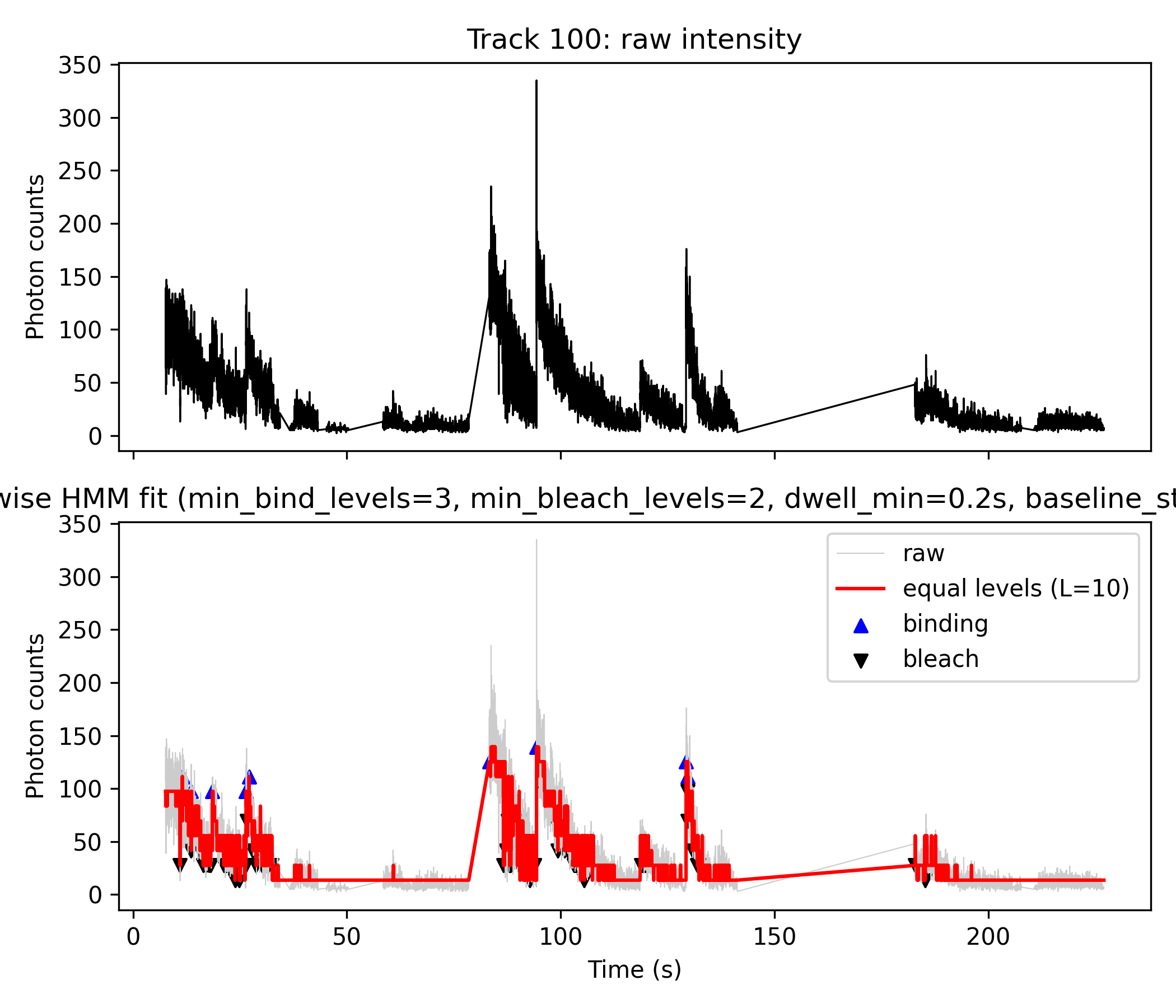
To quantify the molecular assembly of mNeonGreen-labeled LT (mN-LT) proteins on DNA substrates, we implemented a custom Hidden Markov Model (HMM) analysis workflow, closely paralleling approaches previously established for photobleaching-based stoichiometry estimation (see [reference]). Our analysis leverages the fact that photobleaching of individual fluorophores produces quantized, stepwise decreases in integrated fluorescence intensity. By statistically resolving these steps, we infer the number and stability of mN-LT complexes assembled on single DNA molecules.
1. HMM Analysis and Stepwise Discretization: Raw intensity trajectories were extracted for each DNA molecule and analyzed using the ICON algorithm to fit a continuous-time HMM. The resulting mean trajectory, \$ m{mod}(t) \$, was discretized into \$ L \$ equally spaced intensity levels (typically \$ L=10 \$), yielding a stepwise trace, \$ z{step}(t) \$. Each plateau in this trace approximates a molecular “N-mer” state (i.e., with N active fluorophores), while downward steps represent photobleaching events.
2. Event Detection and Thresholding: To robustly define binding and bleaching events, we implemented the following criteria: a binding event is identified as an upward jump of at least three intensity levels (\$ \Delta \geq 3 $), starting from a baseline state of ≤5; bleaching events are defined as downward jumps of at least two levels ($ \Delta \leq -2 $). Dwell time filtering ($ dwell_{min} = 0.2\, s \$) was applied, recursively removing short-lived binding–bleaching episodes to minimize contributions from transient blinking or unreliable detections.
3. Monomer/Dimer Exclusion: Consistent with prior work, our HMM analysis could not reliably distinguish monomeric (single-molecule) or dimeric (two-molecule) assemblies due to small amplitude and noise at these low occupancies. Therefore, binding events corresponding to 1-mer and 2-mer states were excluded from quantitative aggregation, and our statistical interpretation focuses on assemblies of three or more mN-LT molecules.
4. Distribution and Stability Analysis: Event tables were constructed by compiling all detected binding and bleaching episodes across up to 30 DNA molecules and 300+ events. The apparent stoichiometry of mN-LT assemblies ranged principally from 3-mer to 14-mer states, with notable maxima at 3-mer (~32%) and 12-mer (~22%), paralleling DNA double-hexamer formation. Rare occurrences of intermediates (e.g., 10-mer or 11-mer) may reflect rapid cooperative transitions to the most stable 12-mer complexes. Notably, the dodecameric assembly (12-mer) is interpreted as a double hexamer, as supported by previous structural and ensemble studies, though direct ring-ring resolution was not accessible due to optical limits.
5. DNA Sequence Dependence and Controls: Wild-type (WT) Ori98 DNA supported robust 12-mer (double hexamer) assembly across binding events. In contrast, Ori98.Rep—bearing a PS7 mutation—never showed 12-mer formation (n=178 events), with assembly restricted to ≤6–8 mN-LT, consistent with disruption of one hexamer nucleation site. This differential stoichiometry was further validated by size-exclusion chromatography and qPCR on nuclear extracts.
6. Binding Lifetimes by Stoichiometry: Mean dwell times for assembly states were extracted, revealing markedly increased stability with higher-order assemblies. The 3-mer and 6-mer states exhibited mean lifetimes of 36 s and 88 s, respectively, while 12-mers exceeded 1500 s—over 17-fold more stable than single hexamers. These measurements were conducted under active-flow to preclude reassembly artifacts.
7. Correspondence to Present Analysis: Our current pipeline follows a near-identical logic:
8. Software and Reproducibility: All intensity traces were processed using the ICON HMM scripts in Octave/MATLAB, with subsequent discretization and event detection implemented in Python. Complete code and workflow commands are provided in the supplementary materials.
This formulation retains all core technical details: double hexamer assembly, stepwise photobleaching strategy, monomer/dimer filtering, state distribution logic, sequence controls, dwell time quantification, and the direct logic links between your pipeline and the referenced published methodology.
To quantify the assembly of mNeonGreen-labeled LT (mN-LT) proteins on DNA, we constructed an automated workflow based on Hidden Markov Model (HMM) segmentation of single-molecule fluorescence intensity trajectories. This approach utilizes the property that each photobleaching event yields a stepwise, quantized intensity decrease, enabling reconstruction of the number of LT subunits present on the DNA.
First, fluorescence intensity data from individual molecules or foci were modeled using an HMM (ICON algorithm), yielding a denoised mean trajectory \$ m{mod}(t) \$. This trajectory was discretized into \$ L \$ equally spaced intensity levels, matching the expected single-fluorophore step size, to produce a segmented, stepwise intensity trace (\$ z{step}(t) \$). Each plateau in the trace reflected a state with a specific number of active fluorophores (N-mers), while downward steps corresponded to successive photobleaching events.
Binding and bleaching events were automatically detected:
Due to limited resolution, HMM step amplitudes for monomer and dimer states could not be reliably distinguished from noise, so only events representing ≥3 bound LT molecules were included in further quantification (consistent with prior literature). Multimer distributions were then compiled from all detected events, typically ranging from 3-mer to 14-mer, with 12-mer “double hexamer” complexes as a prominent, highly stable state; rare intermediates (10- or 11-mer) likely reflected rapid cooperative assembly into higher order structures. Parallel analysis of wild-type and mutant origins demonstrated nucleation site dependence for 12-mer assembly. Binding dwell times were quantified for each stoichiometry and increased with N, with 12-mer complexes showing dramatically extended stability.
This HMM-based approach thus enables automated, objective quantification of DNA–protein assembly stoichiometry and kinetics using high-throughput, single-molecule photobleaching trajectories.
具体流程如下: 首先,对每一个分子的光强轨迹进行 HMM (ICON 算法) 拟合,得到一个去噪的均值轨迹 \$ m{mod}(t) \$。将此轨迹离散为 \$ L \$ 等间距台阶(对应单分子漂白的幅度),得到分段常数的 step-wise 曲线(\$ z{step}(t) \$)。各平台高度对应于指定数量(N-mer)的 mN-LT,向下台阶代表一个荧光蛋白分子的漂白。
结合与漂白事件的自动检测逻辑为:
由于分子数为1/2的台阶幅度与噪声幅度接近,本方法无法可靠地区分单体和二聚体的组装阶段,因此所有统计仅计入≥3个亚基的结合事件。最终统计出的多聚体分布从3-mer到14-mer不等,其中 12-mer (即 double hexamer)最为显著且稳定(如 Fig. 4C 红/蓝柱所示);10-mer、11-mer等中间体极为罕见,原因可能是组装过程高度协作性,迅速跃迁到高阶结构。对比野生型和突变型 DNA 可揭示核化位点对双六聚体形成的依赖性。不同 N 值的多聚体 binding dwell(结合寿命)也可自动统计,发现 N 越大,寿命越长,12-mer 远高于 single hexamer。
该 HMM 分析流程可实现 DNA–蛋白结合构象的全自动、高通量定量,并为动力学机制研究提供单分子分辨率的坚实基础。] 123456789
https://medcraveonline.com/BBIJ/hidden-markov-model-approaches-for-biological-studies.html ↩
https://www.bakerlab.org/wp-content/uploads/2016/06/bystroff00A.pdf ↩
https://www.research-collection.ethz.ch/bitstreams/d4628f7b-731b-4dc1-8acb-f8ec4ad36541/download ↩
https://umu.diva-portal.org/smash/get/diva2:141606/FULLTEXT01.pdf ↩
“What is confirmed is hexamer and double-hexamer binding to DNA, whereas monomer/dimer binding to DNA is not confirmed.”
This workflow robustly detects and quantifies molecular binding and bleaching events from single-molecule fluorescence trajectories. It employs Hidden Markov Model (HMM) analysis to convert noisy intensity data into interpretable discrete state transitions, using a combination of MATLAB/Octave and Python scripts.
icon_from_track_csv.m, loading each track’s photon count data, fitting a HMM (via the ICON algorithm), and saving results (icon_analysis_track_XX.mat).m_mod)for track_id in 0 1 2 3 4 5 6 7 8 9 10 11 12 13 14; do
octave icon_post_equal_levels.m icon_analysis_track_${track_id}.mat
doneicon_post_equal_levels.m to generate equal_levels_track_XX.mat, which contains a stepwise, discretized version of the HMM fit.for track_id in 0 1 2 3 4 5 6 7 8 9 10 11 12 13 14; do
octave icon_post_equal_levels.m icon_analysis_track_${track_id}.mat
done
# 生成 equal_levels_track_100.mat for Step 4plot_fig4AB_python.pyicon_analysis_track_XX_matlab.mat produced by Step 1.L_best).min_levels_bind=3, min_levels_bleach=2, dwell_min=0.2s, baseline_state_max=5mamba activate kymo_plots
for track_id in 0 1 2 3 4 5 6 7 8 9 10 11 12 13 14 100; do
python plot_fig4AB_python.py ${track_id} 10 3 2 0.2 5
doneicon_multimer_histogram.m is prepared for future use to aggregate results from many tracks (e.g., make multimer/stoichiometry histograms).octave icon_multimer_histogram.m
# for subset use:
octave icon_multimer_histogram.m "equal_levels_track_1*.mat"
#→ 得到 multimer_histogram.png, 就是你的 Fig. 4C-like 图.z).
m_mod) from Step 1 directly inside the python script.Note:
L_best was given directly with 10, was not calculated from Step 2, therefore Step 2 was not used.1. icon_from_track_csv.m (Octave/MATLAB)
2. plot_fig4AB_python.py (Python)
.mat results: time (t), photons (z), and HMM means (m_mod).(Script excerpt, see full file for details):
def assign_to_levels(m_mod, levels):
    # Map every m_mod value to the nearest discrete level
    ...

def detect_binding_bleach_from_state(...):
    # Identify up/down steps using given jump sizes and baseline cutoff
    ...

def filter_short_episodes_by_dwell(...):
    # Filter events with insufficient dwell time
    ...
...
if __name__ == "__main__":
# Parse command line args, load .mat, process and plotSee attached files for full script code:
icon_from_track_csv.mplot_fig4AB_python.pyicon_post_equal_levels.m (diagnostic, not used for current figures)icon_multimer_histogram.m (future)The python script automatically produces a CSV/Excel file summarizing:
In summary:
plot_fig4AB_python.py directly visualize both binding and bleaching events as blue (▲) and black (▼) markers, using logic based on HMM analysis and transition detection within the Python code, without any direct dependence on Step 2 “equal_levels” files. This approach is both robust and reproducible for detailed single-molecule state analysis.
[^1][^2]icon_from_track_csv.m
clear all;
%% icon_from_track_csv.m
%% 用 ICON HMM 分析你自己的 track_intensity CSV 数据
%%
%% 用法(命令行):
%%   octave icon_from_track_csv.m your_track_intensity_file.csv [track_id]
%%
%% - your_track_intensity_file.csv:
%%     3 列分号分隔:
%%     # track index;time (seconds);track intensity (photon counts)
%% - track_id(可选):
%%     要分析的 track_index 数值,例如 0、2、10、100 等
%%     如果不给,则自动:
%%       - 若存在 track 100,则用 100
%%       - 否则用第一个 track

%%--------------------------------------------
%% 0. 处理命令行参数
%%--------------------------------------------
arg_list = argv();
if numel(arg_list) < 1
    error("Usage: octave icon_from_track_csv.m
<track_intensity_csv> [track_id]");
end

input_file = arg_list{1};
track_id_arg = NaN;
if numel(arg_list) >= 2
    track_id_arg = str2double(arg_list{2});
end

fprintf("Input CSV : %s\n", input_file);
if ~isnan(track_id_arg)
    fprintf("Requested track_id: %g\n", track_id_arg);
end

%% 链接 ICON sampler 的源码
%addpath('sampler_SRC');

% 尝试加载 statistics 包(gamrnd 在这里)
try
    pkg load statistics;
catch
    warning("Could not load 'statistics' package. Please install it via 'pkg install -forge statistics'.");
end

%%--------------------------------------------
%% 1. 读入 3 列 CSV: track_index;time;counts
%%--------------------------------------------
fid = fopen(input_file, 'r');
if fid < 0
    error("Cannot open file: %s", input_file);
end

% 第一行是注释头 "# track index;time (seconds);track intensity (photon counts)"
header_line = fgetl(fid);  %#ok
<NASGU>

% 后面每行: track_index;time_sec;intensity
data = textscan(fid, "%f%f%f", "Delimiter", ";");
fclose(fid);

track_idx = data{1};
time_sec  = data{2};
counts    = data{3};

% 按 track 和时间排序,保证序列有序
[~, order] = sortrows([track_idx, time_sec], [1, 2]);
track_idx = track_idx(order);
time_sec  = time_sec(order);
counts    = counts(order);

tracks = unique(track_idx);
fprintf("Found %d tracks: ", numel(tracks));
fprintf("%g ", tracks);
fprintf("\n");

%%--------------------------------------------
%% 2. 选择要分析的 track
%%--------------------------------------------
if ~isnan(track_id_arg)
    tr = track_id_arg;
else
    % 如果存在 track 100,则优先选 100(你自己定义的 accumulated 轨迹)
    if any(tracks == 100)
        tr = 100;
    else
        tr = tracks(1);   % 否则就选第一个
    end
end

if ~any(tracks == tr)
    error("Requested track_id = %g not found in file.", tr);
end

fprintf("Using track_id = %g for ICON analysis.\n", tr);

sel = (track_idx == tr);
t   = time_sec(sel);
z   = counts(sel);

% 按时间排序(理论上已经排过一次,这里再保险)
[ t, order_t ] = sort(t);
z = z(order_t);

z = z(:);  % 列向量
N = numel(z);
fprintf("Track %g has %d time points.\n", tr, N);

%%--------------------------------------------
%% 3. 设置 ICON 参数(与原始脚本一致)
%%--------------------------------------------

% 浓度(Dirichlet 相关超参数)
opts.a = 1;   % Transitions (alpha)
opts.g = 1;   % Base (gamma)

% 超参数 Q
opts.Q(1) = mean(z);         % mean of means (lambda)
opts.Q(2) = 1 / std(z)^2;    % Precision of means (rho)
opts.Q(3) = 0.1;             % Shape of precisions (beta)
opts.Q(4) = 0.00001;         % Scale of precisions (omega)

opts.M = 10;                 % Nodes in the interpolation

% 采样器参数
opts.dr_sk  = 1;             % Stride: 每多少步保存一次 sample
opts.K_init = 50;            % 初始 photon levels 数量(ICON 会自动收缩)

% 输出标志
flag_stat = true;            % 在命令行里打印进度
flag_anim = false;            % 是否弹出动画(Octave 下可以改成 false 更稳定)

%%--------------------------------------------
%% 4. 运行 ICON 采样器
%%--------------------------------------------
R = 1000;   % 样本数,可按需要调整

fprintf("Running ICON sampler on track %g ...\n", tr);
chain = chainer_main( z, R, [], opts, flag_stat, flag_anim );

%%--------------------------------------------
%% 5. 导出 samples 方便后处理
%%--------------------------------------------
fr = 0.25;   % burn-in 比例(前 25%% 样本丢掉)
dr = 2;      % sample stride(每隔多少个样本导出一个)

out_prefix = sprintf('samples_track_%g', tr);
chainer_export(chain, fr, dr, out_prefix, 'mat');
fprintf("Samples exported to %s.mat\n", out_prefix);

%%--------------------------------------------
%% 6. 基本后验分析:state trajectory / transitions / drift
%%--------------------------------------------

% 离散化 state space (在 [0,1] 上划分 25 个 bin)
m_min = 0;
m_max = 1;
m_num = 25;

% (1) 状态轨迹(归一化):m_mod
[m_mod, m_red] = chainer_analyze_means(chain, fr, dr, m_min, m_max, m_num, z);

% (2) 转移概率
[m_edges, p_mean, d_dist] = chainer_analyze_transitions( ...
    chain, fr, dr, m_min, m_max, m_num, true);

% (3) 漂移轨迹
[y_mean, y_std] = chainer_analyze_drift(chain, fr, dr, z);

% 1) Load the original Octave .mat file
%load('icon_analysis_track_100.mat');
% 2) Re-save in MATLAB-compatible v5/v7 format, with new name
%save('-mat', 'icon_analysis_track_100_matlab.mat');

%% 存到一个 mat 文件里,方便之后画图
%icon_mat = sprintf('icon_analysis_track_%g.mat', tr);
%save(icon_mat, 't', 'z', 'm_mod', 'm_red', 'm_edges', 'p_mean', ...
%               'd_dist', 'y_mean', 'y_std');

% 原来的 Octave 版本(可留可不留)
mat_out = sprintf("icon_analysis_track_%d.mat", tr);
save(mat_out, "m_mod", "m_red", "m_edges", "p_mean", "d_dist", ...
              "y_mean", "y_std", "t", "z");

% 额外保存一个专门给 Python / SciPy 用的 MATLAB-compatible 版本
mat_out_matlab = sprintf("icon_analysis_track_%d_matlab.mat", tr);
save('-mat', mat_out_matlab, "m_mod", "m_red", "m_edges", "p_mean", "d_dist", ...
                          "y_mean", "y_std", "t", "z");

fprintf("ICON analysis saved to %s\n", icon_mat);

fprintf("Done.\n");
icon_post_equal_levels.m
% icon_post_equal_levels.m  (script version)
%
% 用法(终端):
%   octave icon_post_equal_levels.m icon_analysis_track_XXX.mat
%
% 对 ICON 分析结果 (icon_analysis_track_XXX.mat) 做等间距 photon level 后处理

arg_list = argv();
if numel(arg_list) < 1
    error("Usage: octave icon_post_equal_levels.m icon_analysis_track_XXX.mat");
end

mat_file = arg_list{1};

fprintf("Loading ICON analysis file: %s\n", mat_file);
S = load(mat_file);

if ~isfield(S, 'm_mod') || ~isfield(S, 't') || ~isfield(S, 'z')
    error("File %s must contain variables: t, z, m_mod.", mat_file);
end

t     = S.t(:);
z     = S.z(:);
m_mod = S.m_mod(:);

N = numel(m_mod);
if numel(t) ~= N || numel(z) ~= N
    error("t, z, m_mod must have the same length.");
end

% 从文件名里解析 track_id(如果有)
[~, name, ~] = fileparts(mat_file);
track_id = NaN;
tokens = regexp(name, 'icon_analysis_track_([0-9]+)', 'tokens');
if ~isempty(tokens)
    track_id = str2double(tokens{1}{1});
    fprintf("Detected track_id = %g from file name.\n", track_id);
else
    fprintf("Could not parse track_id from file name, set to NaN.\n");
end

%--------------------------------------------
% 1. 在 m_mod 的范围上搜索等间距 level 数 L
%--------------------------------------------
m_min = min(m_mod);
m_max = max(m_mod);
fprintf("m_mod range: [%.4f, %.4f]\n", m_min, m_max);

L_min = 2;
L_max = 12;   % 可以按需要改大一些

best_score = Inf;
L_best     = L_min;

fprintf("Scanning candidate level numbers L = %d .. %d ...\n", L_min, L_max);

for L = L_min:L_max
    levels = linspace(m_min, m_max, L);

    % 把每个 m_mod(t) 映射到最近的 level:state_temp ∈ {1..L}
    state_temp = assign_to_levels(m_mod, levels);

    % 用这些 level 生成 step-wise 轨迹
    m_step_temp = levels(state_temp);

    % 计算拟合误差 SSE(在归一化空间)
    residual = m_mod - m_step_temp;
    sse = sum(residual.^2);

    % 类 BIC 评分:误差 + 惩罚 L
    score = N * log(sse / N + eps) + L * log(N);

    fprintf("  L = %2d -> SSE = %.4g, score = %.4g\n", L, sse, score);

    if score < best_score
        best_score = score;
        L_best     = L;
    end
end

fprintf("Best L (number of equally spaced levels) = %d\n", L_best);

%--------------------------------------------
% 2. 用最优 L_best 构建最终的等间距 level & state
%--------------------------------------------
levels_norm = linspace(m_min, m_max, L_best);
state       = assign_to_levels(m_mod, levels_norm);   % 1..L_best
m_step      = levels_norm(state);                     % 归一化台阶轨迹

%--------------------------------------------
% 3. 将归一化台阶轨迹线性映射回 photon counts
%    z ≈ a * m_step + b  (最小二乘)
%--------------------------------------------
A = [m_step(:), ones(N,1)];
theta = A \ z;        % 最小二乘拟合 [a; b]
a = theta(1);
b = theta(2);
z_step = A * theta;   % 拟合出来的 photon counts 台阶轨迹

fprintf("Fitted z ≈ a * m_step + b with a = %.4f, b = %.4f\n", a, b);

%--------------------------------------------
% 4. 检测 bleaching 步:state 下降的时刻
%--------------------------------------------
%s_prev = state(1:end-1);
%s_next = state(2:end);
%
%bleach_idx   = find(s_next < s_prev) + 1;
%bleach_times = t(bleach_idx);
%
%fprintf("Found %d bleaching step(s).\n", numel(bleach_idx));

%--------------------------------------------
% Detect upward (binding) and downward (bleach) steps
%--------------------------------------------
s_prev = state(1:end-1);
s_next = state(2:end);

% raw step indices
bind_idx_raw   = find(s_next > s_prev) + 1;  % upward jumps
bleach_idx_raw = find(s_next < s_prev) + 1;  % downward jumps

% Optional: threshold by intensity change to ignore tiny noisy steps
dz = z_step(2:end) - z_step(1:end-1);

min_jump = 30;   % <-- choose something ~ one level step or larger
keep_bind   = dz >  min_jump;
keep_bleach = dz < -min_jump;

bind_idx   = bind_idx_raw(keep_bind(bind_idx_raw-1));
bleach_idx = bleach_idx_raw(keep_bleach(bleach_idx_raw-1));

bind_times   = t(bind_idx);
bleach_times = t(bleach_idx);

fprintf("Found %d binding and %d bleaching steps (with threshold %.1f).\n", ...
        numel(bind_idx), numel(bleach_idx), min_jump);

%--------------------------------------------
% 5. 保存结果
%--------------------------------------------
out_name = sprintf('equal_levels_track_%s.mat', ...
                   ternary(isnan(track_id), 'X', num2str(track_id)));

fprintf("Saving equal-level analysis to %s\n", out_name);

% Save them in the .mat file
%save(out_name, ...
%     't', 'z', 'm_mod', ...
%     'L_best', 'levels_norm', ...
%     'state', 'm_step', 'z_step', ...
%     'bleach_idx', 'bleach_times', ...
%     'track_id');
save(out_name, ...
     't', 'z', 'm_mod', ...
     'L_best', 'levels_norm', ...
     'state', 'm_step', 'z_step', ...
     'bind_idx', 'bind_times', ...
     'bleach_idx', 'bleach_times', ...
     'track_id');

fprintf("Done.\n");
plot_fig4AB_python.py
#!/usr/bin/env python3
"""
plot_fig4AB_python.py

Usage:
    python plot_fig4AB_python.py
<track_id> [L_best] [min_levels_bind] [min_levels_bleach] [dwell_min] [baseline_state_max]

Arguments
---------

<track_id> : int
    e.g. 10 → uses icon_analysis_track_10_matlab.mat

[L_best]  : int, optional
    Number of equally spaced levels to use for the step-wise fit
    in Fig. 4B. If omitted, default = 3.

[min_levels_bind] : int, optional
    Minimum number of state levels for an upward jump to count as a
    binding event. Default = 3.

[min_levels_bleach] : int, optional
    Minimum number of state levels for a downward jump to count as a
    bleaching step. Default = 1.

[dwell_min] : float, optional
    Minimum allowed dwell time between a binding event and the NEXT
    bleaching event. If Δt = t_bleach - t_bind < dwell_min, then:
        - that binding is removed
        - the paired bleaching event is also removed
    Default = 0 (no dwell-based filtering).

[baseline_state_max] : int, optional
    Highest state index (0-based) that is still considered "baseline /
    unbound" before a binding jump.
    Binding condition becomes:
        dstate >= min_levels_bind  AND  state_before <= baseline_state_max
    If omitted → no baseline constraint (any state can be a start).

Input file
----------
icon_analysis_track_
<track_id>_matlab.mat

Expected variables inside the .mat file:
    t      : time vector (1D, seconds)
    z      : photon counts (1D)
    m_mod  : ICON mean trajectory (1D), same length as t and z

Outputs
-------
1) Figure:
    fig4AB_track_
<track_id>_L<L_best>.png

2) Event tables:
    binding_bleach_events_track_
<track_id>_L<L_best>.csv
    binding_bleach_events_track_
<track_id>_L<L_best>.xlsx   (if pandas available)
"""

import sys
import os
import numpy as np
import matplotlib.pyplot as plt
from scipy.io import loadmat

# Try to import pandas for Excel output
try:
    import pandas as pd
    HAS_PANDAS = True
except ImportError:
    HAS_PANDAS = False
    print("[WARN] pandas not available: Excel output (.xlsx) will be skipped.")

def assign_to_levels(m_mod, levels):
    """
    Map each point in m_mod to the nearest level.

    Parameters
    ----------
    m_mod : array-like, shape (N,)
        Normalized ICON mean trajectory.
    levels : array-like, shape (L,)
        Candidate level values.

    Returns
    -------
    state : ndarray, shape (N,)
        Integer state indices in {0, 1, ..., L-1}.
    """
    m_mod = np.asarray(m_mod).ravel()
    levels = np.asarray(levels).ravel()
    diff = np.abs(m_mod[:, None] - levels[None, :])  # (N, L)
    state = np.argmin(diff, axis=1)  # 0..L-1
    return state

def detect_binding_bleach_from_state(
    z_step,
    t,
    state,
    levels,
    min_levels_bind=3,
    min_levels_bleach=1,
    baseline_state_max=None,
):
    """
    Detect binding (big upward state jumps) and bleaching (downward jumps)
    using the discrete state sequence.

    - Binding: large upward jump (>= min_levels_bind) starting from a
      "baseline" state (state_before <= baseline_state_max) if that
      parameter is given.

    - Bleaching: downward jump (<= -min_levels_bleach)

    Parameters
    ----------
    z_step : array-like, shape (N,)
        Step-wise photon counts.
    t : array-like, shape (N,)
        Time vector (seconds).
    state : array-like, shape (N,)
        Integer states 0..L-1 from assign_to_levels().
    levels : array-like, shape (L,)
        Level values (in m_mod space, not directly photon counts).
    min_levels_bind : int
        Minimum number of levels for an upward jump to be
        considered a binding event.
    min_levels_bleach : int
        Minimum number of levels for a downward jump to be
        considered a bleaching event.
    baseline_state_max : int or None
        Highest state index considered "baseline" before binding.
        If None, any state can be the start of a binding jump.

    Returns
    -------
    bind_idx, bleach_idx : np.ndarray of indices
    bind_times, bleach_times : np.ndarray of times (seconds)
    bind_values, bleach_values : np.ndarray of photon counts at those events
    bind_state_before, bind_state_after : np.ndarray of integer states
    bleach_state_before, bleach_state_after : np.ndarray of integer states
    """

    z_step = np.asarray(z_step).ravel()
    t = np.asarray(t).ravel()
    state = np.asarray(state).ravel()
    levels = np.asarray(levels).ravel()

    N = len(t)
    dstate = np.diff(state)  # length N-1
    idx = np.arange(N - 1)

    # ----- Binding: big upward jump, optionally from baseline only -----
    bind_mask = (dstate >= min_levels_bind)
    if baseline_state_max is not None:
        bind_mask &= (state[idx] <= baseline_state_max)

    bind_idx = idx[bind_mask] + 1

    # ----- Bleaching: downward jump -----
    bleach_mask = (dstate <= -min_levels_bleach)
    bleach_idx = idx[bleach_mask] + 1

    bind_times = t[bind_idx]
    bleach_times = t[bleach_idx]

    bind_values = z_step[bind_idx]
    bleach_values = z_step[bleach_idx]

    bind_state_before = state[bind_idx - 1]
    bind_state_after = state[bind_idx]

    bleach_state_before = state[bleach_idx - 1]
    bleach_state_after = state[bleach_idx]

    return (
        bind_idx,
        bleach_idx,
        bind_times,
        bleach_times,
        bind_values,
        bleach_values,
        bind_state_before,
        bind_state_after,
        bleach_state_before,
        bleach_state_after,
    )

def filter_short_episodes_by_dwell(
    bind_idx,
    bleach_idx,
    bind_times,
    bleach_times,
    bind_values,
    bleach_values,
    bind_state_before,
    bind_state_after,
    bleach_state_before,
    bleach_state_after,
    dwell_min,
):
    """
    Remove short binding episodes based on dwell time and also remove
    the paired bleaching step.

    Rule:
        For each binding, find the first bleaching with t_bleach > t_bind.
        If Δt = t_bleach - t_bind < dwell_min, then:
            - remove this binding
            - remove this bleaching
        All other bleaching events remain.

    Returns
    -------
    (filtered binding arrays, dwell_times) + filtered bleaching arrays
    """

    if dwell_min <= 0 or len(bind_idx) == 0 or len(bleach_idx) == 0:
        # no filtering requested or missing events
        dwell_times = np.full(len(bind_idx), np.nan)
        for i in range(len(bind_idx)):
            future = np.where(bleach_times > bind_times[i])[0]
            if len(future) > 0:
                dwell_times[i] = bleach_times[future[0]] - bind_times[i]
        return (
            bind_idx,
            bleach_idx,
            bind_times,
            bleach_times,
            bind_values,
            bleach_values,
            bind_state_before,
            bind_state_after,
            bleach_state_before,
            bleach_state_after,
            dwell_times,
        )

    bind_idx = np.asarray(bind_idx)
    bleach_idx = np.asarray(bleach_idx)
    bind_times = np.asarray(bind_times)
    bleach_times = np.asarray(bleach_times)
    bind_values = np.asarray(bind_values)
    bleach_values = np.asarray(bleach_values)
    bind_state_before = np.asarray(bind_state_before)
    bind_state_after = np.asarray(bind_state_after)
    bleach_state_before = np.asarray(bleach_state_before)
    bleach_state_after = np.asarray(bleach_state_after)

    keep_bind = np.ones(len(bind_idx), dtype=bool)
    keep_bleach = np.ones(len(bleach_idx), dtype=bool)
    dwell_times = np.full(len(bind_idx), np.nan)

    removed_bind = 0
    removed_bleach = 0

    for i in range(len(bind_idx)):
        t_b = bind_times[i]
        future = np.where(bleach_times > t_b)[0]
        if len(future) == 0:
            # no bleaching afterwards → dwell undefined, keep binding
            dwell_times[i] = np.nan
            continue

        j = future[0]
        dt = bleach_times[j] - t_b
        dwell_times[i] = dt

        if dt < dwell_min:
            # remove this binding and its paired bleaching
            keep_bind[i] = False
            if keep_bleach[j]:
                keep_bleach[j] = False
                removed_bleach += 1
            removed_bind += 1

    print(
        f"[INFO] Dwell-based filter: removed {removed_bind} binding(s) and "
        f"{removed_bleach} paired bleaching step(s) with Δt < {dwell_min} s; "
        f"{np.sum(keep_bind)} binding(s) and {np.sum(keep_bleach)} bleaching step(s) kept."
    )

    # Apply masks
    bind_idx = bind_idx[keep_bind]
    bind_times = bind_times[keep_bind]
    bind_values = bind_values[keep_bind]
    bind_state_before = bind_state_before[keep_bind]
    bind_state_after = bind_state_after[keep_bind]
    dwell_times = dwell_times[keep_bind]

    bleach_idx = bleach_idx[keep_bleach]
    bleach_times = bleach_times[keep_bleach]
    bleach_values = bleach_values[keep_bleach]
    bleach_state_before = bleach_state_before[keep_bleach]
    bleach_state_after = bleach_state_after[keep_bleach]

    return (
        bind_idx,
        bleach_idx,
        bind_times,
        bleach_times,
        bind_values,
        bleach_values,
        bind_state_before,
        bind_state_after,
        bleach_state_before,
        bleach_state_after,
        dwell_times,
    )

def plot_fig4AB(
    track_id,
    L_best=None,
    min_levels_bind=3,
    min_levels_bleach=1,
    dwell_min=0.0,
    baseline_state_max=None,
):
    # --------------------------
    # 1. Load ICON analysis file
    # --------------------------
    mat_file = f"icon_analysis_track_{track_id}_matlab.mat"
    print(f"Loading {mat_file}")
    if not os.path.exists(mat_file):
        raise FileNotFoundError(f"{mat_file} does not exist in current directory.")

    data = loadmat(mat_file)

    def extract_vector(name):
        if name not in data:
            raise KeyError(f"Variable '{name}' not found in {mat_file}")
        v = data[name]
        return np.squeeze(v)

    t = extract_vector("t")
    z = extract_vector("z")
    m_mod = extract_vector("m_mod")

    if not (len(t) == len(z) == len(m_mod)):
        raise ValueError("t, z, and m_mod must have the same length.")

    N = len(t)
    print(f"Track {track_id}: N = {N} points")

    # --------------------------
    # 2. Choose L (number of levels)
    # --------------------------
    if L_best is None:
        L_best = 3  # fallback default
        print(f"No L_best provided, using default L_best = {L_best}")
    else:
        print(f"Using user-specified L_best = {L_best}")

    m_min = np.min(m_mod)
    m_max = np.max(m_mod)
    levels = np.linspace(m_min, m_max, L_best)
    print(f"m_mod range: [{m_min:.4f}, {m_max:.4f}]")
    print(f"Equally spaced levels ({L_best}): {levels}")

    # --------------------------
    # 3. Build step-wise trajectory from m_mod
    # --------------------------
    state = assign_to_levels(m_mod, levels)  # 0..L_best-1
    m_step = levels[state]

    # Map back to photon counts via linear fit z ≈ a*m_step + b
    A = np.column_stack([m_step, np.ones(N)])
    theta, *_ = np.linalg.lstsq(A, z, rcond=None)
    a, b = theta
    z_step = A @ theta
    print(f"Fitted z ≈ a * m_step + b with a = {a:.4f}, b = {b:.4f}")

    # --------------------------
    # 4. Detect binding / bleaching events (state-based)
    # --------------------------
    (
        bind_idx,
        bleach_idx,
        bind_times,
        bleach_times,
        bind_values,
        bleach_values,
        bind_state_before,
        bind_state_after,
        bleach_state_before,
        bleach_state_after,
    ) = detect_binding_bleach_from_state(
        z_step,
        t,
        state,
        levels,
        min_levels_bind=min_levels_bind,
        min_levels_bleach=min_levels_bleach,
        baseline_state_max=baseline_state_max,
    )

    base_msg = (
        f"baseline_state_max={baseline_state_max}"
        if baseline_state_max is not None
        else "baseline_state_max=None (no baseline restriction)"
    )
    print(
        f"Initial detection: {len(bind_idx)} binding and {len(bleach_idx)} bleaching "
        f"events (min_levels_bind={min_levels_bind}, "
        f"min_levels_bleach={min_levels_bleach}, {base_msg})."
    )

    # --------------------------
    # 5. Apply dwell-time filter to binding + paired bleach
    # --------------------------
    (
        bind_idx,
        bleach_idx,
        bind_times,
        bleach_times,
        bind_values,
        bleach_values,
        bind_state_before,
        bind_state_after,
        bleach_state_before,
        bleach_state_after,
        dwell_times,
    ) = filter_short_episodes_by_dwell(
        bind_idx,
        bleach_idx,
        bind_times,
        bleach_times,
        bind_values,
        bleach_values,
        bind_state_before,
        bind_state_after,
        bleach_state_before,
        bleach_state_after,
        dwell_min=dwell_min,
    )

    print(
        f"After dwell filter (dwell_min={dwell_min}s): "
        f"{len(bind_idx)} binding and {len(bleach_idx)} bleaching events remain."
    )

    # --------------------------
    # 6. Build event table & save CSV / Excel
    # --------------------------
    rows = []

    # Binding events
    for i in range(len(bind_idx)):
        idx = int(bind_idx[i])
        rows.append({
            "event_type": "binding",
            "sample_index": idx,
            "time_seconds": float(bind_times[i]),
            "photon_count": float(bind_values[i]),
            "state_before": int(bind_state_before[i]),
            "state_after": int(bind_state_after[i]),
            "level_before_norm": float(levels[bind_state_before[i]]),
            "level_after_norm": float(levels[bind_state_after[i]]),
            "dwell_time": float(dwell_times[i]) if not np.isnan(dwell_times[i]) else "",
        })

    # Bleaching events
    for i in range(len(bleach_idx)):
        idx = int(bleach_idx[i])
        rows.append({
            "event_type": "bleach",
            "sample_index": idx,
            "time_seconds": float(bleach_times[i]),
            "photon_count": float(bleach_values[i]),
            "state_before": int(bleach_state_before[i]),
            "state_after": int(bleach_state_after[i]),
            "level_before_norm": float(levels[bleach_state_before[i]]),
            "level_after_norm": float(levels[bleach_state_after[i]]),
            "dwell_time": "",
        })

    # Sort by time
    rows = sorted(rows, key=lambda r: r["time_seconds"])

    # Write CSV
    csv_name = f"binding_bleach_events_track_{track_id}_L{L_best}.csv"
    import csv
    with open(csv_name, "w", newline="") as f:
        writer = csv.DictWriter(
            f,
            fieldnames=[
                "event_type",
                "sample_index",
                "time_seconds",
                "photon_count",
                "state_before",
                "state_after",
                "level_before_norm",
                "level_after_norm",
                "dwell_time",
            ],
        )
        writer.writeheader()
        for r in rows:
            writer.writerow(r)

    print(f"Saved event table to {csv_name}")

    # Write Excel (if pandas available)
    if HAS_PANDAS:
        df = pd.DataFrame(rows)
        xlsx_name = f"binding_bleach_events_track_{track_id}_L{L_best}.xlsx"
        df.to_excel(xlsx_name, index=False)
        print(f"Saved event table to {xlsx_name}")
    else:
        print("[INFO] pandas not installed → skipped Excel (.xlsx) output.")

    # --------------------------
    # 7. Make a figure similar to Fig. 4A + 4B
    # --------------------------
    fig, axes = plt.subplots(2, 1, figsize=(7, 6), sharex=True)

    # ---- Fig. 4A-like: raw intensity vs time ----
    ax1 = axes[0]
    ax1.plot(t, z, color="black", linewidth=0.8)
    ax1.set_ylabel("Photon counts")
    ax1.set_title(f"Track {track_id}: raw intensity")  #(Fig. 4A-like)

    # ---- Fig. 4B-like: step-wise HMM fit vs time ----
    ax2 = axes[1]
    ax2.plot(t, z, color="0.8", linewidth=0.5, label="raw")
    ax2.plot(t, z_step, color="red", linewidth=1.5,
             label=f"equal levels (L={L_best})")

    # Mark binding (up-steps) and bleaching (down-steps) AFTER filtering
    if len(bind_idx) > 0:
        ax2.scatter(
            bind_times,
            bind_values,
            marker="^",
            color="blue",
            s=30,
            label="binding",
        )
    if len(bleach_idx) > 0:
        ax2.scatter(
            bleach_times,
            bleach_values,
            marker="v",
            color="black",
            s=30,
            label="bleach",
        )

    ax2.set_xlabel("Time (s)")
    ax2.set_ylabel("Photon counts")
    ax2.set_title(
        f"Step-wise HMM fit ("    #Fig. 4B-like,
        f"min_bind_levels={min_levels_bind}, "
        f"min_bleach_levels={min_levels_bleach}, "
        f"dwell_min={dwell_min}s, "
        f"baseline_state_max={baseline_state_max})"
    )
    ax2.legend(loc="best")

    fig.tight_layout()
    out_png = f"fig4AB_track_{track_id}_L{L_best}.png"
    fig.savefig(out_png, dpi=300)
    plt.close(fig)
    print(f"Saved figure to {out_png}")

if __name__ == "__main__":
    if len(sys.argv) < 2:
        print("Usage: python plot_fig4AB_python.py
<track_id> [L_best] [min_levels_bind] [min_levels_bleach] [dwell_min] [baseline_state_max]")
        sys.exit(1)

    track_id = int(sys.argv[1])

    # Defaults
    L_best = None
    min_levels_bind = 3
    min_levels_bleach = 1
    dwell_min = 0.0
    baseline_state_max = None

    if len(sys.argv) >= 3:
        L_best = int(sys.argv[2])
    if len(sys.argv) >= 4:
        min_levels_bind = int(sys.argv[3])
    if len(sys.argv) >= 5:
        min_levels_bleach = int(sys.argv[4])
    if len(sys.argv) >= 6:
        dwell_min = float(sys.argv[5])
    if len(sys.argv) >= 7:
        baseline_state_max = int(sys.argv[6])

    plot_fig4AB(
        track_id,
        L_best=L_best,
        min_levels_bind=min_levels_bind,
        min_levels_bleach=min_levels_bleach,
        dwell_min=dwell_min,
        baseline_state_max=baseline_state_max,
    )
icon_multimer_histogram.m
% icon_multimer_histogram.m
%
% 用法(终端):
%   octave icon_multimer_histogram.m [pattern]
%
% 默认 pattern = "equal_levels_track_*.mat"
%
% 要求每个 mat 文件里至少有:
%   state      : 等间距 level 的索引 (1..L_best)
%   t          : 时间向量
%   z          : 原始 photon counts
%   track_id   : (可选) 轨迹编号,用于打印信息
%
% 输出:
%   - 在命令行打印每条轨迹估计出的 multimer 数目
%   - 生成 Fig. 4C 风格直方图:
%       multimer_histogram.png

arg_list = argv();
if numel(arg_list) >= 1
    pattern = arg_list{1};
else
    pattern = "equal_levels_track_*.mat";
end

fprintf("Searching files with pattern: %s\n", pattern);
files = dir(pattern);

if isempty(files)
    error("No files matched pattern: %s", pattern);
end

multimers = [];      % 保存每条轨迹的 multimer size
track_ids = [];      % 保存对应的 track_id(若存在)

fprintf("Found %d files.\n", numel(files));

for i = 1:numel(files)
    fname = files(i).name;
    fprintf("\nLoading %s ...\n", fname);
    S = load(fname);

    if ~isfield(S, "state") || ~isfield(S, "t")
        warning("  File %s does not contain 'state' or 't'. Skipped.", fname);
        continue;
    end

    state = S.state(:);
    t     = S.t(:);

    N = numel(state);
    if N < 5
        warning("  File %s has too few points (N=%d). Skipped.", fname, N);
        continue;
    end

    % 解析 track_id(如果有)
    tr_id = NaN;
    if isfield(S, "track_id")
        tr_id = S.track_id;
    else
        % 尝试从文件名里解析
        tokens = regexp(fname, 'equal_levels_track_([0-9]+)', 'tokens');
        if ~isempty(tokens)
            tr_id = str2double(tokens{1}{1});
        end
    end

    % 取前 10%% 和后 10%% 时间段的 state 中位数
    n_head = max(1, round(0.1 * N));
    n_tail = max(1, round(0.1 * N));

    head_idx = 1:n_head;
    tail_idx = (N - n_tail + 1):N;

    initial_state = round(median(state(head_idx)));
    final_state   = round(median(state(tail_idx)));

    multimer_size = initial_state - final_state;

    if multimer_size <= 0
        fprintf("  Track %g: initial_state=%d, final_state=%d -> multimer_size=%d (ignored)\n", ...
                tr_id, initial_state, final_state, multimer_size);
        continue;
    end

    fprintf("  Track %g: initial_state=%d, final_state=%d -> multimer_size=%d\n", ...
            tr_id, initial_state, final_state, multimer_size);

    multimers(end+1,1) = multimer_size;
    track_ids(end+1,1) = tr_id;
end

if isempty(multimers)
    error("No valid multimer sizes estimated. Check your data or thresholds.");
end

% 像论文那样,可以选择去掉 monomer/dimer
fprintf("\nTotal %d events (including monomer/dimer).\n", numel(multimers));

% 可选:过滤掉 ≤2 的(monomer / dimer)
mask = multimers > 2;
multimers_filtered = multimers(mask);
fprintf("After removing monomer/dimer (<=2): %d events.\n", numel(multimers_filtered));

if isempty(multimers_filtered)
    error("No events left after filtering monomer/dimer. Try including them.");
end

% 计算直方图
max_mult = max(multimers_filtered);
edges = 0.5:(max_mult + 0.5);
[counts, edges_out] = histcounts(multimers_filtered, edges);
centers = 1:max_mult;

% 画 Fig. 4C 风格的柱状图
figure;
bar(centers, counts, 'FaceColor', [0.2 0.6 0.8]); % 颜色随便,Octave 会忽略
xlabel('Number of mN-LT per origin (multimer size)');
ylabel('Frequency');
title('Distribution of multimer sizes (Fig. 4C-like)');
xlim([0.5, max_mult + 0.5]);

% 在每个柱子上标一下计数
hold on;
for k = 1:max_mult
    if counts(k) > 0
        text(centers(k), counts(k) + 0.1, sprintf('%d', counts(k)), ...
             'HorizontalAlignment', 'center');
    end
end
hold off;

print('-dpng', 'multimer_histogram.png');
fprintf("\n[INFO] Multimer histogram saved to multimer_histogram.png\n");English: Advances in DNA sequencing have revolutionized biology, but converting vast sequencing data into usable, robust biological knowledge depends on sophisticated bioinformatics. This review details computational strategies spanning all phases of DNA sequence analysis, starting from raw reads through to functional interpretation and reporting. It begins by characterizing the main sequencing platforms (short-read, long-read, targeted, and metagenomic), describes critical pipeline steps (sample tracking, quality control, read alignment, error correction, variant and structural variant detection, copy number analysis, de novo assembly), and considers the impact of reference genome choice and computational algorithms. Recent machine learning advances for variant annotation and integration with other omics are discussed, with applications highlighted in rare disease diagnostics, cancer genomics, and infectious disease surveillance. Emphasis is placed on reproducible, scalable, and well-documented pipelines using open-source tools, workflow management (Snakemake, Nextflow), containerization, versioning, and FAIR data principles. The review concludes with discussion of ongoing challenges (heterogeneous data, batch effects, benchmarking, privacy) and practical recommendations for robust, interpretable analyses for both experimental biologists and computational practitioners.
Chinese: DNA测序的持续进步彻底改变了生物学和医学研究,而要将庞大的测序数据转化为可靠的生物学知识,则高度依赖高水平的生物信息学方法。本文详细介绍了DNA序列分析全流程的主流计算策略,涵盖原始reads到功能性注释乃至标准化报告的各个环节。首先评述主流测序技术平台(短读长读、靶向、宏基因组),系统阐述实验设计、样本追踪、数据质控、比对、纠错、变异与结构变异检测、拷贝数分析和de novo组装等流程要点,并分析参考基因组和比对算法对结果的影响。文章还总结了机器学习在变异注释、多组学整合中的最新进展,结合罕见病诊断、肿瘤基因组和病原体监测等实际案例深入说明其应用场景。着重强调可重复、高效、透明的分析流程,包括开源工具、流程管理(Snakemake、Nextflow)、容器化、版本管理与FAIR原则。最后讨论了异质数据、批次效应、评测标准和隐私保护等挑战,并为实验与计算生物学研究者提供实用建议。
Section Opening (English / 中文): High-throughput DNA sequencing has fundamentally transformed modern genomics, enabling detailed investigation of human diseases, microbial ecology, and evolution. However, the raw output—massive quantities of short or long reads—is only the starting point; extracting meaningful, robust insights requires optimized bioinformatics pipelines that ensure data integrity and biological relevance.
高通量DNA测序极大地推动了现代基因组学,助力人类疾病、微生物生态与进化等领域的深入探索。但测序仪输出的原始reads只是起点——要获得有意义、可靠的生物学结论,必须依赖优化的生物信息学流程以保证数据质量和生物学解释的可信度。
Here is a concise bilingual summary of your text explaining the idea and a cleaned-up proposal to send to Vero:
https://www.sciencedirect.com/science/article/pii/S0022283625003742 ↩
https://phys.libretexts.org/Courses/University_of_California_Davis/Biophysics_241:_Membrane_Biology/05:_Experimental_Characterization_-_Spectroscopy_and_Microscopy/5.07:_Single_Molecule_Tracking ↩
https://royalsocietypublishing.org/doi/10.1098/rsob.210383 ↩
% detect_binding_bleach.m
% 用法(在终端):
%   octave detect_binding_bleach.m p853_250706_p502_10pN_ch5_0bar_b3_1_track_intensity_data_blue_5s.csv

%--------------------------------------------
% 基本设置
%--------------------------------------------
arg_list = argv();
if numel(arg_list) < 1
    error("Usage: octave detect_binding_bleach.m
<track_intensity_csv>");
end
input_file = arg_list{1};

% 加载 HMM 采样器
%addpath("sampler_SRC");

% 如果安装了 statistics 包,用于 kmeans
try
    pkg load statistics;
catch
    warning("Could not load 'statistics' package. Make sure it is installed if kmeans is missing.");
end

%--------------------------------------------
% 读入 track intensity 文件(分号分隔)
%--------------------------------------------
fprintf("Reading file: %s\n", input_file);

fid = fopen(input_file, "r");
if fid < 0
    error("Cannot open file: %s", input_file);
end

% 第一行是注释头 "# track index;time (seconds);track intensity (photon counts)"
header_line = fgetl(fid);  % 忽略内容,只是读掉这一行

% 后面每行: track_index;time_sec;intensity
data = textscan(fid, "%f%f%f", "Delimiter", ";");
fclose(fid);

track_idx = data{1};
time_sec  = data{2};
counts    = data{3};

% 排序(确保同一个 track 内按时间排序)
[~, order] = sortrows([track_idx, time_sec], [1, 2]);
track_idx = track_idx(order);
time_sec  = time_sec(order);
counts    = counts(order);

tracks = unique(track_idx);
n_tracks = numel(tracks);

fprintf("Found %d tracks.\n", n_tracks);

%--------------------------------------------
% 结果结构体
%--------------------------------------------
results = struct( ...
    "track_id", {}, ...
    "binding_indices", {}, ...
    "binding_times", {}, ...
    "bleach_indices", {}, ...
    "bleach_times", {} );

%--------------------------------------------
% 循环每个 track,跑 HMM + 找事件
%--------------------------------------------
for ti = 1:n_tracks
    tr = tracks(ti);
    fprintf("\n===== Track %d =====\n", tr);

    sel = (track_idx == tr);
    t = time_sec(sel);
    z = counts(sel);
    z = z(:);      % 列向量

    %-------------------------
    % 1) 设定 ICON HMM 的参数
    %-------------------------
    opts = struct();

    % 超参数(和原 MATLAB 代码一致)
    opts.a = 1;
    opts.g = 1;

    opts.Q(1) = mean(z);
    opts.Q(2) = 1 / (std(z)^2 + eps);   % 防止除零
    opts.Q(3) = 0.1;
    opts.Q(4) = 0.00001;

    opts.M = 10;

    % 采样参数
    opts.dr_sk  = 1;
    opts.K_init = 50;

    flag_stat = true;
    flag_anim = false;    % 建议在 Octave 里关掉动画更稳定

    R = 1000;             % 采样次数,可根据需要调小/调大

    %-------------------------
    % 2) 运行采样器
    %-------------------------
    fprintf("  Running HMM sampler...\n");
    chain = chainer_main(z, R, [], opts, flag_stat, flag_anim);

    %-------------------------
    % 3) 做后验分析,得到平滑后的光子水平轨迹
    %-------------------------
    fr = 0.25;        % burn-in 比例
    dr = 2;           % sample 步距

    m_min = 0;
    m_max = 1;
    m_num = 25;

    [m_mod, m_red] = chainer_analyze_means(chain, fr, dr, m_min, m_max, m_num, z);

    % m_mod 是一个和 z 同长度的向量(通常是 [0,1] 范围的归一化水平)
    m_mod = m_mod(:);

    %-------------------------
    % 4) 把 m_mod 聚类成 3 个光子强度状态
    %    状态 1 = 最低强度 (dark / unbound / bleached)
    %    状态 3 = 最高强度 (bound)
    %-------------------------
    K = 3;   % 你可以改成 2 或其他
    try
        [idx_raw, centers] = kmeans(m_mod, K);
    catch
        % 如果没 kmeans,就简单按数值分位数来分三类
        warning("kmeans not available, using simple quantile-based clustering.");
        q1 = quantile(m_mod, 1/3);
        q2 = quantile(m_mod, 2/3);
        idx_raw = ones(size(m_mod));
        idx_raw(m_mod > q1 & m_mod <= q2) = 2;
        idx_raw(m_mod > q2) = 3;
        centers = zeros(K,1);
        for kk = 1:K
            centers(kk) = mean(m_mod(idx_raw == kk));
        end
    end

    % 根据中心值从小到大重排状态编号
    [~, order_centers] = sort(centers);
    state_seq = zeros(size(idx_raw));
    for k = 1:K
        state_seq(idx_raw == order_centers(k)) = k;
    end

    low_state  = 1;
    high_state = K;

    %-------------------------
    % 5) 检测 binding / bleach 跳变
    %    binding:  low -> high
    %    bleach : high -> low
    %-------------------------
    s = state_seq(:);
    % 前一时刻和后一时刻
    s_prev = s(1:end-1);
    s_next = s(2:end);

    bind_idx   = find(s_prev == low_state  & s_next == high_state) + 1;
    bleach_idx = find(s_prev == high_state & s_next == low_state) + 1;

    bind_times   = t(bind_idx);
    bleach_times = t(bleach_idx);

    fprintf("  Found %d binding event(s) and %d bleaching event(s).\n", ...
            numel(bind_idx), numel(bleach_idx));

    % 存入结果
    results(ti).track_id        = tr;
    results(ti).binding_indices = bind_idx;
    results(ti).binding_times   = bind_times;
    results(ti).bleach_indices  = bleach_idx;
    results(ti).bleach_times    = bleach_times;
end

%--------------------------------------------
% 6) 把结果写成 CSV
%--------------------------------------------
out_csv = "binding_bleach_events.csv";
fid_out = fopen(out_csv, "w");
if fid_out < 0
    error("Cannot open output file: %s", out_csv);
end

fprintf(fid_out, "track_index,event_type,sample_index,time_seconds\n");
for ti = 1:numel(results)
    tr = results(ti).track_id;

    % binding
    for k = 1:numel(results(ti).binding_indices)
        fprintf(fid_out, "%d,binding,%d,%.6f\n", tr, ...
                results(ti).binding_indices(k), ...
                results(ti).binding_times(k));
    end

    % bleach
    for k = 1:numel(results(ti).bleach_indices)
        fprintf(fid_out, "%d,bleach,%d,%.6f\n", tr, ...
                results(ti).bleach_indices(k), ...
                results(ti).bleach_times(k));
    end
end
fclose(fid_out);

fprintf("\nAll done. Events written to: %s\n", out_csv);octave detect_binding_bleach.m p853_250706_p502_10pN_ch5_0bar_b3_1_track_intensity_data_blue_5s.csvchainer_export 导出样本chainer_analyze_means 得到 m_modchainer_analyze_transitions 得到 m_edges, p_mean, d_distchainer_analyze_drift 得到 y_mean, y_std说明:
- 代码仍然基于你已有的
detect_binding_bleach.m结构,假定当前目录下有sampler_SRC(含chainer_main.m、chainer_analyze_means.m、chainer_analyze_transitions.m、chainer_analyze_drift.m等)。1819- Dwell time 这里使用“连续 binding 事件之间的时间差”来估计 bound-state dwell time(简化版);如果 bleaching 明确是轨迹末端终止,也可以用
bleach_time - last_binding_time作为一个 right‑censored dwell(这里暂不做 censoring 修正,只输出原始分布和单指数拟合)。
detect_binding_bleach_dwell_simple.m% detect_binding_bleach_dwell.m
%
% 用法(终端):
% octave detect_binding_bleach_dwell.m p853_250706_p502_10pN_ch5_0bar_b3_1_track_intensity_data_blue_5s.csv
%
% 输入 CSV 格式(分号分隔):
% # track index;time (seconds);track intensity (photon counts)
% 1;0.00;123
% 1;0.05;118
% 2;0.00; 95
% ...
%--------------------------------------------
% 0. 基本设置
%--------------------------------------------
arg_list = argv();
if numel(arg_list) < 1
error("Usage: octave detect_binding_bleach_dwell.m
<input_csv>");
end
input_file = arg_list{1};
% 加载 HMM 采样器代码(确保 sampler_SRC 在当前目录下)
addpath("sampler_SRC");
% 如果安装了 statistics 包,用于 kmeans
try
pkg load statistics;
catch
warning("Could not load 'statistics' package. Make sure it is installed if kmeans is missing.");
end
%--------------------------------------------
% 1. 读入 track intensity 文件(分号分隔)
%--------------------------------------------
fprintf("Reading file: %s\n", input_file);
fid = fopen(input_file, "r");
if fid < 0
error("Cannot open file: %s", input_file);
end
% 第一行是注释头 "# track index;time (seconds);track intensity (photon counts)"
header_line = fgetl(fid); % 忽略内容,只是读掉这一行
% 后面每行: track_index;time_sec;intensity
data = textscan(fid, "%f%f%f", "Delimiter", ";");
fclose(fid);
track_idx = data{1};
time_sec = data{2};
counts = data{3};
% 排序(确保同一个 track 内按时间排序)
[~, order] = sortrows([track_idx, time_sec], [1, 2]);
track_idx = track_idx(order);
time_sec = time_sec(order);
counts = counts(order);
tracks = unique(track_idx);
n_tracks = numel(tracks);
fprintf("Found %d tracks.\n", n_tracks);
%--------------------------------------------
% 2. 结果结构体(binding / bleach 时间点)
%--------------------------------------------
results = struct( ...
"track_id", {}, ...
"binding_indices", {}, ...
"binding_times", {}, ...
"bleach_indices", {}, ...
"bleach_times", {} );
% 用于 dwell time 收集的数组
all_binding_times = []; % 所有 track 的 binding time 合并
all_bleach_times = []; % 所有 track 的 bleach time 合并
%--------------------------------------------
% 3. 循环每个 track,跑 HMM + ICON 分析 + 事件检测
%--------------------------------------------
for ti = 1:n_tracks
tr = tracks(ti);
fprintf("\n===== Track %d =====\n", tr);
sel = (track_idx == tr);
t = time_sec(sel);
z = counts(sel);
z = z(:); % 列向量
%-------------------------
% 3.1 设定 ICON HMM 的参数
%-------------------------
opts = struct();
% 超参数(与 level_analysis.m 一致)
opts.a = 1;
opts.g = 1;
opts.Q(1) = mean(z);
opts.Q(2) = 1 / (std(z)^2 + eps); % 防止 std(z)=0 除零
opts.Q(3) = 0.1;
opts.Q(4) = 0.00001;
opts.M = 10;
% 采样参数
opts.dr_sk = 1;
opts.K_init = 50;
flag_stat = true;
flag_anim = false; % 建议在 Octave 里关掉动画
R = 1000; % 采样次数,可按需求调整
%-------------------------
% 3.2 运行采样器(ICON HMM)
%-------------------------
fprintf(" Running HMM sampler...\n");
chain = chainer_main(z, R, [], opts, flag_stat, flag_anim);
%-------------------------
% 3.3 ICON 后验分析(与 level_analysis.m 等价)
%-------------------------
fr = 0.25; % burn-in 比例
dr = 2; % sample 步距
m_min = 0;
m_max = 1;
m_num = 25;
% (1) 均值轨迹:m_mod
[m_mod, m_red] = chainer_analyze_means(chain, fr, dr, m_min, m_max, m_num, z);
m_mod = m_mod(:);
% (2) 导出 samples(为每条 track 单独存一个文件)
sample_file = sprintf("samples_track_%d", tr);
chainer_export(chain, fr, dr, sample_file, "mat");
% (3) 转移概率 / 跃迁统计
[m_edges, p_mean, d_dist] = chainer_analyze_transitions( ...
chain, fr, dr, m_min, m_max, m_num, true);
% (4) 漂移分析
[y_mean, y_std] = chainer_analyze_drift(chain, fr, dr, z);
% 你可以根据需要保存这些 ICON 分析结果
mat_out = sprintf("icon_analysis_track_%d.mat", tr);
save(mat_out, "m_mod", "m_red", "m_edges", "p_mean", "d_dist", ...
"y_mean", "y_std", "t", "z");
%-------------------------
% 3.4 把 m_mod 聚类成 3 个光子强度状态(用于事件检测)
%-------------------------
K = 3; % 可按物理需求修改
try
[idx_raw, centers] = kmeans(m_mod, K);
catch
warning("kmeans not available, using simple quantile-based clustering.");
q1 = quantile(m_mod, 1/3);
q2 = quantile(m_mod, 2/3);
idx_raw = ones(size(m_mod));
idx_raw(m_mod > q1 & m_mod <= q2) = 2;
idx_raw(m_mod > q2) = 3;
centers = zeros(K,1);
for kk = 1:K
centers(kk) = mean(m_mod(idx_raw == kk));
end
end
% 根据中心值从小到大重排状态编号,使 state_seq = 1..K 对应 low->high
[~, order_centers] = sort(centers);
state_seq = zeros(size(idx_raw));
for k = 1:K
state_seq(idx_raw == order_centers(k)) = k;
end
low_state = 1;
high_state = K;
%-------------------------
% 3.5 检测 binding / bleaching
%
% binding: low_state -> high_state
% bleach : high_state -> low_state
%-------------------------
s = state_seq(:);
s_prev = s(1:end-1);
s_next = s(2:end);
bind_idx = find(s_prev == low_state & s_next == high_state) + 1;
bleach_idx = find(s_prev == high_state & s_next == low_state) + 1;
bind_times = t(bind_idx);
bleach_times = t(bleach_idx);
fprintf(" Found %d binding event(s) and %d bleaching event(s).\n", ...
numel(bind_idx), numel(bleach_idx));
% 存入结果结构体
results(ti).track_id = tr;
results(ti).binding_indices = bind_idx;
results(ti).binding_times = bind_times;
results(ti).bleach_indices = bleach_idx;
results(ti).bleach_times = bleach_times;
% 用于全局 dwell-time 统计
all_binding_times = [all_binding_times; bind_times(:)];
all_bleach_times = [all_bleach_times; bleach_times(:)];
end
%--------------------------------------------
% 4. 输出 binding/bleach 时间点的总表(最重要输出)
%--------------------------------------------
out_csv = "binding_bleach_events.csv";
fid_out = fopen(out_csv, "w");
if fid_out < 0
error("Cannot open output file: %s", out_csv);
end
fprintf(fid_out, "track_index,event_type,sample_index,time_seconds\n");
for ti = 1:numel(results)
tr = results(ti).track_id;
% binding
for k = 1:numel(results(ti).binding_indices)
fprintf(fid_out, "%d,binding,%d,%.6f\n", tr, ...
results(ti).binding_indices(k), ...
results(ti).binding_times(k));
end
% bleach
for k = 1:numel(results(ti).bleach_indices)
fprintf(fid_out, "%d,bleach,%d,%.6f\n", tr, ...
results(ti).bleach_indices(k), ...
results(ti).bleach_times(k));
end
end
fclose(fid_out);
fprintf("\n[INFO] Binding/bleach events written to: %s\n", out_csv);
%--------------------------------------------
% 5. Dwell-time 直方图 + rate 拟合
%
% 简化假设:
% - 把每个 track 中连续 binding 事件之间的时间差视为
% bound state dwell time(中间没有 bleaching,就重新 binding)。
% - 如果有明确的最后一个 binding 到 bleaching 的时间,
% 你也可以扩展这里把它们当作 dwell time 加进去。
%--------------------------------------------
% 5.1 收集 bound-state dwell times(简单用 binding 时间差)
dwell_times = [];
for ti = 1:numel(results)
bt = sort(results(ti).binding_times(:)); % 单个 track 的 binding times
if numel(bt) >= 2
dt = diff(bt); % 相邻 binding 之间的时间差
dwell_times = [dwell_times; dt];
end
% 可选:如果你想把最后一个 binding -> 第一个 bleach 也算入 dwell:
% if ~isempty(results(ti).binding_times) && ~isempty(results(ti).bleach_times)
% last_binding = max(results(ti).binding_times);
% first_bleach = min(results(ti).bleach_times);
% if first_bleach > last_binding
% dwell_times = [dwell_times; first_bleach - last_binding];
% end
% end
end
if isempty(dwell_times)
fprintf("[WARN] No sufficient binding events to compute dwell-time distribution.\n");
else
% 5.2 绘制 dwell-time 直方图
figure;
hold on;
nbins = max(10, round(sqrt(numel(dwell_times)))); % 简单经验 bin 数
[counts_hist, edges] = histcounts(dwell_times, nbins);
centers = (edges(1:end-1) + edges(2:end)) / 2;
bar(centers, counts_hist, "hist");
xlabel("Dwell time (s)");
ylabel("Counts");
title("Bound-state dwell-time histogram");
% 5.3 拟合单指数: p(t) ~ (1/tau) * exp(-t/tau)
% 使用简单的最小二乘拟合 log(count) 对 t
valid = counts_hist > 0;
t_fit = centers(valid);
y_fit = log(counts_hist(valid));
% 线性拟合: log(N) = a + b * t, 其中 b ~= -1/tau
p = polyfit(t_fit, y_fit, 1);
a = p(1);
b = p(2);
tau_est = -1 / b;
fprintf("[INFO] Fitted single-exponential dwell time tau = %.4f s\n", tau_est);
% 画出拟合曲线(归一到 histogram 的总 counts 约束)
t_plot = linspace(min(dwell_times), max(dwell_times), 200);
% 预测密度 ~ exp(a + b t),但我们要匹配 histogram 的离散计数
y_model = exp(a + b * t_plot);
plot(t_plot, y_model, "r-", "LineWidth", 2);
legend("Histogram", "Single-exp fit");
hold off;
% 可选:保存图像
print("-dpng", "dwell_time_histogram_fit.png");
fprintf("[INFO] Dwell-time histogram and fit saved to dwell_time_histogram_fit.png\n");
end
fprintf("\nAll done.\n");octave detect_binding_bleach_dwell_simple.m p853_250706_p502_10pN_ch5_0bar_b3_1_track_intensity_data_blue_5s.csv会生成:
binding_bleach_events.csv:所有 track 的 binding/bleach 时间点(你最关心的表格)。icon_analysis_track_X.mat:每个 track 的 ICON 分析结果(m_mod, m_edges, p_mean, d_dist, y_mean, y_std 等)。dwell_time_histogram_fit.png,包含 dwell-time 直方图和单指数拟合曲线。last_binding -> first_bleach 的逻辑打开或进一步改写成更严格的两态 dwell 定义。tau_est 是平均 dwell time,解离 rate 大致是 $k{\text{off}} = 1/\tau{\text{est}}$。如果你需要可以在脚本里再打印一条 k_off_est。如果你希望 dwell-time 统计严格区分 “bound state dwell vs unbound state dwell”,或者想直接从 p_mean / d_dist 中做 rate 矩阵估计,可以在这份脚本基础上再往前一步;可以一起设计一个更“教科书版”的 HMM‑rate 推断流程。
特性概览:
chainer_main)分析每个 track。18level_analysis.m 的四类后验分析:chainer_export、chainer_analyze_means、chainer_analyze_transitions、chainer_analyze_drift。18m_mod 聚类成 3 个强度状态,检测 binding / bleaching 事件。19binding_bleach_events.csv,包含所有 binding/bleach 时间点。19print + close 保存 PNG(类似 R 的 dev.off()),并使用 hist 而不是 histcounts。19将以下内容保存为 detect_binding_bleach_dwell.m 即可直接运行。
detect_binding_bleach_dwell.m 完整代码% detect_binding_bleach_dwell.m
%
% 用法(终端):
% octave detect_binding_bleach_dwell.m p853_250706_p502_10pN_ch5_0bar_b3_1_track_intensity_data_blue_5s.csv
%
% 输入 CSV 格式(分号分隔):
% # track index;time (seconds);track intensity (photon counts)
% 1;0.00;123
% 1;0.05;118
% 2;0.00; 95
% ...
%--------------------------------------------
% 0. 基本设置
%--------------------------------------------
arg_list = argv();
if numel(arg_list) < 1
error("Usage: octave detect_binding_bleach_dwell.m
<input_csv>");
end
input_file = arg_list{1};
% 加载 HMM 采样器代码(确保 sampler_SRC 在当前目录下)
addpath("sampler_SRC");
% 如果安装了 statistics 包,用于 kmeans
try
pkg load statistics;
catch
warning("Could not load 'statistics' package. Make sure it is installed if kmeans is missing.");
end
%--------------------------------------------
% 1. 读入 track intensity 文件(分号分隔)
%--------------------------------------------
fprintf("Reading file: %s\n", input_file);
fid = fopen(input_file, "r");
if fid < 0
error("Cannot open file: %s", input_file);
end
% 第一行是注释头 "# track index;time (seconds);track intensity (photon counts)"
header_line = fgetl(fid); % 忽略内容,只是读掉这一行
% 后面每行: track_index;time_sec;intensity
data = textscan(fid, "%f%f%f", "Delimiter", ";");
fclose(fid);
track_idx = data{1};
time_sec = data{2};
counts = data{3};
% 排序(确保同一个 track 内按时间排序)
[~, order] = sortrows([track_idx, time_sec], [1, 2]);
track_idx = track_idx(order);
time_sec = time_sec(order);
counts = counts(order);
tracks = unique(track_idx);
n_tracks = numel(tracks);
fprintf("Found %d tracks.\n", n_tracks);
%--------------------------------------------
% 2. 结果结构体(binding / bleach 时间点)
%--------------------------------------------
results = struct( ...
"track_id", {}, ...
"binding_indices", {}, ...
"binding_times", {}, ...
"bleach_indices", {}, ...
"bleach_times", {} );
% 用于 dwell time 收集的数组(跨所有 track)
all_binding_times = []; % 所有 track 的 binding time 合并
all_bleach_times = []; % 所有 track 的 bleach time 合并
%--------------------------------------------
% 3. 循环每个 track,跑 HMM + ICON 分析 + 事件检测
%--------------------------------------------
for ti = 1:n_tracks
tr = tracks(ti);
fprintf("\n===== Track %d =====\n", tr);
sel = (track_idx == tr);
t = time_sec(sel);
z = counts(sel);
z = z(:); % 列向量
%-------------------------
% 3.1 设定 ICON HMM 的参数
%-------------------------
opts = struct();
% 超参数(与 level_analysis.m 一致)
opts.a = 1;
opts.g = 1;
opts.Q(1) = mean(z);
opts.Q(2) = 1 / (std(z)^2 + eps); % 防止 std(z)=0 除零
opts.Q(3) = 0.1;
opts.Q(4) = 0.00001;
opts.M = 10;
% 采样参数
opts.dr_sk = 1;
opts.K_init = 50;
flag_stat = true;
flag_anim = false; % 建议在 Octave 里关掉动画
R = 1000; % 采样次数,可按需求调整
%-------------------------
% 3.2 运行采样器(ICON HMM)
%-------------------------
fprintf(" Running HMM sampler...\n");
chain = chainer_main(z, R, [], opts, flag_stat, flag_anim);
%-------------------------
% 3.3 ICON 后验分析(与 level_analysis.m 等价)
%-------------------------
fr = 0.25; % burn-in 比例
dr = 2; % sample 步距
m_min = 0;
m_max = 1;
m_num = 25;
% (1) 均值轨迹:m_mod
[m_mod, m_red] = chainer_analyze_means(chain, fr, dr, m_min, m_max, m_num, z);
m_mod = m_mod(:);
% (2) 导出 samples(为每条 track 单独存一个文件)
sample_file = sprintf("samples_track_%d", tr);
chainer_export(chain, fr, dr, sample_file, "mat");
fprintf("%s --- Exported\n", [sample_file ".mat"]);
% (3) 转移概率 / 跃迁统计
[m_edges, p_mean, d_dist] = chainer_analyze_transitions( ...
chain, fr, dr, m_min, m_max, m_num, true);
% (4) 漂移分析
[y_mean, y_std] = chainer_analyze_drift(chain, fr, dr, z);
% 保存这些 ICON 分析结果(可选)
mat_out = sprintf("icon_analysis_track_%d.mat", tr);
save(mat_out, "m_mod", "m_red", "m_edges", "p_mean", "d_dist", ...
"y_mean", "y_std", "t", "z");
%-------------------------
% 3.4 把 m_mod 聚类成 3 个光子强度状态(用于事件检测)
%-------------------------
K = 3; % 可按物理需求修改
try
[idx_raw, centers] = kmeans(m_mod, K);
catch
warning("kmeans not available, using simple quantile-based clustering.");
q1 = quantile(m_mod, 1/3);
q2 = quantile(m_mod, 2/3);
idx_raw = ones(size(m_mod));
idx_raw(m_mod > q1 & m_mod <= q2) = 2;
idx_raw(m_mod > q2) = 3;
centers = zeros(K,1);
for kk = 1:K
centers(kk) = mean(m_mod(idx_raw == kk));
end
end
% 根据中心值从小到大重排状态编号,使 state_seq = 1..K 对应 low->high
[~, order_centers] = sort(centers);
state_seq = zeros(size(idx_raw));
for k = 1:K
state_seq(idx_raw == order_centers(k)) = k;
end
low_state = 1;
high_state = K;
%-------------------------
% 3.5 检测 binding / bleaching
%
% binding: low_state -> high_state
% bleach : high_state -> low_state
%-------------------------
s = state_seq(:);
s_prev = s(1:end-1);
s_next = s(2:end);
bind_idx = find(s_prev == low_state & s_next == high_state) + 1;
bleach_idx = find(s_prev == high_state & s_next == low_state) + 1;
bind_times = t(bind_idx);
bleach_times = t(bleach_idx);
fprintf("Found %d binding event(s) and %d bleaching event(s).\n", ...
numel(bind_idx), numel(bleach_idx));
% 存入结果结构体
results(ti).track_id = tr;
results(ti).binding_indices = bind_idx;
results(ti).binding_times = bind_times;
results(ti).bleach_indices = bleach_idx;
results(ti).bleach_times = bleach_times;
% 用于全局 dwell-time 统计
all_binding_times = [all_binding_times; bind_times(:)];
all_bleach_times = [all_bleach_times; bleach_times(:)];
end
%--------------------------------------------
% 4. 输出 binding/bleach 时间点的总表(最重要输出)
%--------------------------------------------
out_csv = "binding_bleach_events.csv";
fid_out = fopen(out_csv, "w");
if fid_out < 0
error("Cannot open output file: %s", out_csv);
end
fprintf(fid_out, "track_index,event_type,sample_index,time_seconds\n");
for ti = 1:numel(results)
tr = results(ti).track_id;
% binding
for k = 1:numel(results(ti).binding_indices)
fprintf(fid_out, "%d,binding,%d,%.6f\n", tr, ...
results(ti).binding_indices(k), ...
results(ti).binding_times(k));
end
% bleach
for k = 1:numel(results(ti).bleach_indices)
fprintf(fid_out, "%d,bleach,%d,%.6f\n", tr, ...
results(ti).bleach_indices(k), ...
results(ti).bleach_times(k));
end
end
fclose(fid_out);
fprintf("\n[INFO] Binding/bleach events written to: %s\n", out_csv);
%--------------------------------------------
% 5. Dwell-time 直方图 + rate 拟合
%
% 简化假设:
% - 把每个 track 中连续 binding 事件之间的时间差视为
% bound state dwell time(中间没有 bleaching,就重新 binding)。
% - 如果有明确的最后一个 binding 到 bleaching 的时间,
% 可以扩展此处加入(当前先保留简单版本)。
%--------------------------------------------
% 5.1 收集 bound-state dwell times(简单用 binding 时间差)
dwell_times = [];
for ti = 1:numel(results)
bt = sort(results(ti).binding_times(:)); % 单个 track 的 binding times
if numel(bt) >= 2
dt = diff(bt); % 相邻 binding 之间的时间差
dwell_times = [dwell_times; dt];
end
% 可选:如果你想把最后一个 binding -> 第一个 bleach 也算入 dwell:
% if ~isempty(results(ti).binding_times) && ~isempty(results(ti).bleach_times)
% last_binding = max(results(ti).binding_times);
% first_bleach = min(results(ti).bleach_times);
% if first_bleach > last_binding
% dwell_times = [dwell_times; first_bleach - last_binding];
% end
% end
end
if isempty(dwell_times)
fprintf("[WARN] No sufficient binding events to compute dwell-time distribution.\n");
else
% 5.2 绘制 dwell-time 直方图(只在内存中画,不弹窗)
fig = figure("visible", "off");
hold on;
nbins = max(10, round(sqrt(numel(dwell_times))));
% 使用 hist(Octave 自带)代替 histcounts
[counts_hist, centers] = hist(dwell_times, nbins);
bar(centers, counts_hist, "hist");
xlabel("Dwell time (s)");
ylabel("Counts");
title("Bound-state dwell-time histogram");
% 5.3 拟合单指数: p(t) ~ (1/tau) * exp(-t/tau)
valid = counts_hist > 0;
t_fit = centers(valid);
y_fit = log(counts_hist(valid));
p = polyfit(t_fit, y_fit, 1);
a = p(1);
b = p(2);
tau_est = -1 / b;
fprintf("[INFO] Fitted single-exponential dwell time tau = %.4f s\n", tau_est);
t_plot = linspace(min(dwell_times), max(dwell_times), 200);
y_model = exp(a + b * t_plot);
plot(t_plot, y_model, "r-", "LineWidth", 2);
legend("Histogram", "Single-exp fit");
hold off;
% 保存图像并关闭 figure(类似 R 的 dev.off())
out_png = "dwell_time_histogram_fit.png";
print(fig, out_png, "-dpng");
close(fig);
fprintf("[INFO] Dwell-time histogram and fit saved to %s\n", out_png);
end
fprintf("\nAll done.\n");运行方式:
octave detect_binding_bleach_dwell.m p853_250706_p502_10pN_ch5_0bar_b3_1_track_intensity_data_blue_5s.csv如有下一步你想基于 d_dist 做更“纯 HMM”的 dwell 分布 / rate 矩阵,也可以在这个脚本上再加一节专门分析。
这两个脚本在核心 HMM 采样算法上是一致的,但整体流程和用途并不完全相同。level_analysis.m只是做“ICON HMM 拟合 + 若干通用后验分析”,而 detect_binding_bleach.m在此基础上,额外做了“多 track 输入 + 聚类成离散状态 + 自动识别 binding/bleach 跳变 + 输出 CSV”。因此不能说是完全相同算法的简单移植,而是“在相同 HMM 内核上扩展出的一个更完整事件检测流程”。1819
下面分两部分说明:先列出关键差异,然后用中文系统讲解 detect_binding_bleach.m 的整个处理流程(包括和原始 level_analysis.m 共享的 HMM 部分)。1918
level_analysis.m:侧重“通用分析”,调用:
detect_binding_bleach.m:只调用 chainer_analyze_means 得到 m_mod,然后完全走另一条分析线:
结论:
detect_binding_bleach.m 的完整流程(含与原脚本共用的 HMM 思路)下面把 detect_binding_bleach.m 当作主角,用中文分步骤解释其处理流程,并在相关步骤指出它与原 level_analysis.m 的对应关系。这样方便你检查是否满足你对“算法一致性”的期待。1918
argv() 读取命令行参数,第一个参数是输入文件名,例如:
octave detect_binding_bleach.m p853_250706_p502_10pN_ch5_0bar_b3_1_track_intensity_data_blue_5s.csv。19track_index:轨迹编号(一个 DNA tether 或一个粒子)。time_seconds:该轨迹下某一帧的时间点。track_intensity:该时间点的 photon counts。track_idx, time_sec, counts。然后用 sortrows([track_idx, time_sec]) 按 “轨迹号优先,再按时间” 排好顺序,保证每条轨迹都是时间有序的。之后提取所有不同的 tracks,准备对每一条轨迹单独做分析。19这一步在原 level_analysis.m 中要简单得多,那里只是 z = load('photoncount.txt');,默认只处理单一系列,没有 track 结构。18
for ti = 1:n_tracks 遍历每一个 track。tr,用 sel = (track_idx == tr) 挑出这一条轨迹对应的时间和强度,得到:
t = time_sec(sel):该轨迹的时间轴。z = counts(sel):该轨迹的 photon count 序列。z 转成列向量,作为后续 HMM 的观测数据。到这里为止,z 的角色与原脚本中的 z = load('photoncount.txt') 完全一致,只是这里是“多轨迹版本”的 z。1819
这一段是两份脚本的核心重合部分,也是你最关心的“算法一致性”所在。1819
opts 结构体,用于向 chainer_main 传参。opts.a = 1;:控制 HMM 中状态转换的 Dirichlet 浓度(类似“转移稀疏度”的先验强度)。opts.g = 1;:控制状态先验分布的基本参数(base measure 的浓度)。opts.Q(1) = mean(z);:假设状态均值的先验均值等于观测平均值。opts.Q(2) = 1 / (std(z)^2 + eps);:状态均值先验的精度,与观测标准差成反比;加上 eps 是为了避免在极端情形下 std(z) = 0 导致除零。原 MATLAB 版本是 1/std(z)^2,数学上是一致的设定。opts.Q(3) = 0.1;:方差逆数的 Gamma 先验的 shape。opts.Q(4) = 0.00001;:方差逆数的 Gamma 先验的 scale。opts.M = 10;:插值节点数(ICON 模型内部数值近似需要)。opts.dr_sk = 1;:保存样本的间隔步长。opts.K_init = 50;:初始假设的隐状态数(实际有效状态数由采样自动调整)。R = 1000;:采样迭代次数。这些设置在 level_analysis.m 中完全一致,只是缺少 eps。所以从贝叶斯 HMM 模型结构和先验设定来看,两者是同一个 ICON 模型。1918
chain = chainer_main(z, R, [], opts, flag_stat, flag_anim); 来运行 ICON HMM 的 Gibbs sampler 或类似的 MCMC 算法。
chainer_main 内部会对每个时间点的隐状态、每个状态的均值和方差、转移矩阵等进行采样,得到一条或多条后验链 chain,用来近似整个后验分布。这个步骤在两个脚本里完全相同,只是 Octave 版本对可视化做了简化。1918
chainer_analyze_meansfr = 0.25:前 25% 的样本视为 burn-in,丢弃不用。dr = 2:之后每隔 2 个样本取一个,用来减弱自相关。m_min = 0; m_max = 1; m_num = 25;:把状态均值的可能范围离散成 $[0,1]$ 区间上 25 个格点,用于后验平均的插值或投影。[m_mod, m_red] = chainer_analyze_means(chain, fr, dr, m_min, m_max, m_num, z);m_mod 可以理解为“在每一个时间点上的后验平均光子水平”,往往已被归一化到 $[0,1]$ 区间,是一个与 z 等长的一维轨迹。m_red 是某种降维或简化形式,这里没有用到。1819这一部分与 level_analysis.m 完全一致,区别在于:原脚本后面还继续做转移概率估计和漂移分析;Octave 版则转向“离散状态 + 事件检测”。1918
接下来是 Octave 脚本中新加的上层算法部分,用来从连续的 m_mod 中自动提取“低/中/高”强度状态:
K = 3(可手动改成 2 或其他)。kmeans(m_mod, K) 对 m_mod 做聚类,得到:
idx_raw:每个时间点所属的簇编号。centers:每个簇的中心值(大致对应不同光子水平)。kmeans 不可用,就退化为基于分位数的简单阈值法:
q1 = quantile(m_mod, 1/3); q2 = quantile(m_mod, 2/3); 把轨迹分为低、中、高三段。centers。centers 后,按照中心值从小到大排序,重排状态编号,使得:
low_state)。high_state)。这一段在 level_analysis.m 中没有任何对应逻辑,是 Octave 版本为 binding/bleach 检测专门设计的。其本质是:用连续的后验均值轨迹做无监督聚类,把连续空间映射为少数几个离散层级状态。1819
有了状态序列 state_seq 后,就可以做简单的“状态跳变检测”来定义事件:
s = state_seq(:)。s_prev = s(1:end-1);s_next = s(2:end);s_prev == low_state 且 s_next == high_state 时,即从低强度直接跳到高强度,视为一次“分子结合”(binding)。find(...) + 1,因为跳变是在第二个点发生。s_prev == high_state 且 s_next == low_state 时,即从高强度直接掉回低强度,视为一次“光漂白或解离”(bleaching/unbinding)。find(...) + 1。t(bind_idx) 和 t(bleach_idx) 把这些索引转换成真实时间点(秒),分别作为 binding_times 和 bleach_times。这一步把 HMM 的连续后验轨迹,最终转化成了一个离散事件时间列表。在原 level_analysis.m 中,没有这类应用导向的 event detection,只停留在“描述状态分布和转移概率”的层面。1918
for ti = 1:n_tracks 循环内,把每条轨迹的事件信息存入 results(ti):
track_idbinding_indices, binding_timesbleach_indices, bleach_times。19binding_bleach_events.csv,格式为:
track_index,event_type,sample_index,time_secondsevent_type 是 "binding" 或 "bleach"。相较之下,level_analysis.m 用的是 chainer_export 把整条 MCMC 链以 .mat 形式保存,供交互式分析和可视化使用,而不是面向“事件列表”的输出。1819
eps 防止除零,以及关闭动画提高稳定性,这不会改变算法本质。level_analysis.m 是一个“通用 ICON HMM 演示与分析脚本”,只做单一序列的建模和一些统计性后验分析,不涉及具体事件检测逻辑。
detect_binding_bleach.m 在沿用同一 HMM 内核的基础上,增加了:多轨迹处理、对后验均值轨迹的聚类、将轨迹离散为若干强度状态、基于状态跳变的 binding/bleach 自动识别以及 CSV 输出。这是一层新的、面向应用的算法,不存在于原 MATLAB 脚本中。如果你的目标是“在 Octave 中复用原 ICON HMM 的统计建模部分,并进一步实现自动 binding/bleaching 检测”,那么当前 detect_binding_bleach.m 的设计是符合这一思路的:核心推断算法相同,外层分析逻辑则是针对具体实验需求进行了扩展。