Monthly Archives: October 2025

Step‑by‑Step Workflow for Phylogenomic and Functional Analysis of 100 Clinical Isolates Using WGS Data

  • ggtree_and_gheatmap_kpneumoniae_new
  • ggtree_and_gheatmap_paeruginosa_new
  • ggtree_and_gheatmap_paeruginosa
  • ggtree_and_gheatmap_kpneumoniae
  • ggtree_and_gheatmap_abaumannii
  • ggtree_and_gheatmap_ecoli

Below is a sorted, step‑by‑step protocol integrating all commands and materials from your notes — organized into logical analysis phases. It outlines how to process whole‑genome data, annotate with Prokka, perform pan‑genome and SNP‑based phylogenetic analysis, and conduct resistome profiling and visualization.


1. Initial Setup and Environment Configuration

  1. Create and activate working environments:
conda create -n bengal3_ac3 python=3.9
conda activate /home/jhuang/miniconda3/envs/bengal3_ac3
  1. Copy necessary config files for bacto:
cp /home/jhuang/Tools/bacto/bacto-0.1.json .
cp /home/jhuang/Tools/bacto/Snakefile .
  1. Prepare R environment for later visualization:
mamba create -n r_414_bioc314 -c conda-forge -c bioconda \
  r-base=4.1.3 bioconductor-ggtree bioconductor-treeio \
  r-ggplot2 r-dplyr r-ape pandoc

2. Species Assignment and MLST Screening

  • Use WGS data to determine phylogenetic relationships based on MLST. Confirm species identity of isolates: E. coli, K. pneumoniae, A. baumannii complex, P. aeruginosa.
  • Example log output:
[10:19:59] Excluding ecoli.icdA.262 due to --exclude option
[10:19:59] If you like MLST, you're going to absolutely love cgMLST!
[10:19:59] Done.
  • Observation: No strain was close enough to be a suspected clonal strain (to be confirmed later with SNP‑based analysis).

3. Genome Annotation with Prokka

Cluster isolates into four species folders and annotate each genome separately.

Example shell script:

for cluster in abaumannii_2 ecoli_achtman_4 klebsiella paeruginosa; do
  GENUS_MAP=( [abaumannii_2]="Acinetobacter" [ecoli_achtman_4]="Escherichia" [klebsiella]="Klebsiella" [paeruginosa]="Pseudomonas" )
  SPECIES_MAP=( [abaumannii_2]="baumannii" [ecoli_achtman_4]="coli" [klebsiella]="pneumoniae" [paeruginosa]="aeruginosa" )
  prokka --force --outdir prokka/${cluster} --cpus 8 \
         --genus ${GENUS_MAP[$cluster]} --species ${SPECIES_MAP[$cluster]} \
         --addgenes --addmrna --prefix ${cluster} \
         -hmm /media/jhuang/Titisee/GAMOLA2/TIGRfam_db/TIGRFAMs_15.0_HMM.LIB
 done

4. Pan‑Genome Construction with Roary

Run Roary for each species cluster (GFF outputs from Prokka):

roary -f roary/ecoli_cluster -e --mafft -p 100 prokka/ecoli_cluster/*.gff
roary -f roary/kpneumoniae_cluster1 -e --mafft -p 100 prokka/kpneumoniae_cluster1/*.gff
roary -f roary/abaumannii_cluster -e --mafft -p 100 prokka/abaumannii_cluster/*.gff
roary -f roary/paeruginosa_cluster -e --mafft -p 100 prokka/paeruginosa_cluster/*.gff

Output: core gene alignments for each species.


5. Core‑Genome Phylogenetic Tree Building (RAxML‑NG)

Use maximum likelihood reconstruction per species:

raxml-ng --all --msa roary/ecoli_achtman_4/core_gene_alignment.aln --model GTR+G --bs-trees 1000 --threads 40 --prefix ecoli_core_gene_tree_1000
raxml-ng --all --msa roary/klebsiella/core_gene_alignment.aln --model GTR+G --bs-trees 1000 --threads 40 --prefix klebsiella_core_gene_tree_1000
raxml-ng --all --msa roary/abaumannii/core_gene_alignment.aln --model GTR+G --bs-trees 1000 --threads 40 --prefix abaumannii_core_gene_tree_1000
raxml-ng --all --msa roary/paeruginosa/core_gene_alignment.aln --model GTR+G --bs-trees 1000 --threads 40 --prefix paeruginosa_core_gene_tree_1000

6. SNP Detection and Distance Calculation

  1. Extract SNP sites and generate distance matrices:
snp-sites -v -o core_snps.vcf roary/ecoli_achtman_4/core_gene_alignment.aln
snp-dists roary/ecoli_achtman_4/core_gene_alignment.aln > ecoli_snp_dist.tsv
  1. Repeat for other species and convert to Excel summary:
~/Tools/csv2xls-0.4/csv_to_xls.py ecoli_snp_dist.tsv klebsiella_snp_dist.tsv abaumannii_snp_dist.tsv paeruginosa_snp_dist.tsv -d$'\t' -o snp_dist.xls

7. Resistome and Virulence Profiling with Abricate

  1. Install and set up databases:
conda install -c bioconda -c conda-forge abricate=1.0.1
abricate --setupdb
abricate --list
DATABASE        SEQUENCES       DBTYPE  DATE
vfdb    2597    nucl    2025-Oct-22
resfinder       3077    nucl    2025-Oct-22
argannot        2223    nucl    2025-Oct-22
ecoh    597     nucl    2025-Oct-22
megares 6635    nucl    2025-Oct-22
card    2631    nucl    2025-Oct-22
ecoli_vf        2701    nucl    2025-Oct-22
plasmidfinder   460     nucl    2025-Oct-22
ncbi    5386    nucl    2025-Oct-22
  1. Run VFDB for virulence genes:
# # Run VFDB example
# abricate --db vfdb genome.fasta > vfdb.tsv
#
# # strict filter (≥90% ID, ≥80% cov) using header-safe awk
# awk -F'\t' 'NR==1{
#   for(i=1;i<=NF;i++){if($i=="%IDENTITY") id=i; if($i=="%COVERAGE") cov=i}
#   print; next
# } ($id+0)>=90 && ($cov+0)>=80' vfdb.tsv > vfdb.strict.tsv

# 0) Define your cluster directories (exactly as in your prompt)
CLUSTERS="fasta_abaumannii_cluster fasta_kpnaumoniae_cluster1 fasta_kpnaumoniae_cluster2 fasta_kpnaumoniae_cluster3"

# 1) Run Abricate (VFDB) per isolate, strictly filtered (≥90% ID, ≥80% COV)
for D in $CLUSTERS; do
  mkdir -p "$D/abricate_vfdb"
  for F in "$D"/*.fasta; do
    ISO=$(basename "$F" .fasta)
    # raw
    abricate --db vfdb "$F" > "$D/abricate_vfdb/${ISO}.vfdb.tsv"
    # strict filter while keeping header (header-safe awk)
    awk -F'\t' 'NR==1{
      for(i=1;i<=NF;i++){if($i=="%IDENTITY") id=i; if($i=="%COVERAGE") cov=i}
      print; next
    } ($id+0)>=90 && ($cov+0)>=80' \
      "$D/abricate_vfdb/${ISO}.vfdb.tsv" > "$D/abricate_vfdb/${ISO}.vfdb.strict.tsv"
  done
done

# 2) Build per-cluster "isolate
<TAB>gene" lists (Abricate column 5 = GENE)
for D in $CLUSTERS; do
  OUT="$D/virulence_isolate_gene.tsv"
  : > "$OUT"
  for T in "$D"/abricate_vfdb/*.vfdb.strict.tsv; do
    ISO=$(basename "$T" .vfdb.strict.tsv)
    awk -F'\t' -v I="$ISO" 'NR>1{print I"\t"$5}' "$T" >> "$OUT"
  done
  sort -u "$OUT" -o "$OUT"
done

# 3) Create a per-isolate "signature" (sorted, comma-joined gene list)
for D in $CLUSTERS; do
  IN="$D/virulence_isolate_gene.tsv"
  SIG="$D/virulence_signatures.tsv"
  awk -F'\t' '
  {m[$1][$2]=1}
  END{
    for(i in m){
      n=0
      for(g in m[i]){n++; a[n]=g}
      asort(a)
      printf("%s\t", i)
      for(k=1;k<=n;k++){printf("%s%s", (k>1?",":""), a[k])}
      printf("\n")
      delete a
    }
  }' "$IN" | sort > "$SIG"
done

# 4) Report whether each cluster is internally identical
for D in $CLUSTERS; do
  SIG="$D/virulence_signatures.tsv"
  echo "== $D =="
  # how many unique signatures?
  CUT=$(cut -f2 "$SIG" | sort -u | wc -l)
  if [ "$CUT" -eq 1 ]; then
    echo "  Virulence profiles: IDENTICAL within cluster"
  else
    echo "  Virulence profiles: NOT IDENTICAL (unique signatures: $CUT)"
    echo "  --- differing isolates & their signatures ---"
    cat "$SIG"
  fi
done
  1. Summarize VFDB results:
#----
# Make gene lists (VFDB "GENE" = column 5) for each isolate
cut -f5 fasta_kpnaumoniae_cluster2/abricate_vfdb/QRC018.vfdb.strict.tsv | tail -n +2 | sort -u > c2_018.genes.txt
cut -f5 fasta_kpnaumoniae_cluster2/abricate_vfdb/QRC070.vfdb.strict.tsv | tail -n +2 | sort -u > c2_070.genes.txt

# Show symmetric differences
echo "Genes present in QRC018 only:"
comm -23 c2_018.genes.txt c2_070.genes.txt

echo "Genes present in QRC070 only:"
comm -13 c2_018.genes.txt c2_070.genes.txt

awk -F'\t' 'NR>1{print $5"\t"$6}' fasta_kpnaumoniae_cluster2/abricate_vfdb/QRC018.vfdb.strict.tsv | sort -u > c2_018.gene_product.txt
awk -F'\t' 'NR>1{print $5"\t"$6}' fasta_kpnaumoniae_cluster2/abricate_vfdb/QRC070.vfdb.strict.tsv | sort -u > c2_070.gene_product.txt

# Genes unique to QRC018 with product
join -t $'\t' <(cut -f1 c2_018.gene_product.txt) <(cut -f1 c2_070.gene_product.txt) -v1 > /dev/null # warms caches
comm -23 <(cut -f1 c2_018.gene_product.txt | sort) <(cut -f1 c2_070.gene_product.txt | sort) \
  | xargs -I{} grep -m1 -P "^{}\t" c2_018.gene_product.txt

# Genes unique to QRC070 with product
comm -13 <(cut -f1 c2_018.gene_product.txt | sort) <(cut -f1 c2_070.gene_product.txt | sort) \
  | xargs -I{} grep -m1 -P "^{}\t" c2_070.gene_product.txt

# Make a cluster summary table from raw (or strict) TSVs
for D in fasta_abaumannii_cluster fasta_kpnaumoniae_cluster1 fasta_kpnaumoniae_cluster2 fasta_kpnaumoniae_cluster3; do
  echo "== $D =="
  abricate --summary "$D"/abricate_vfdb/*.vfdb.strict.tsv | column -t
done
  1. Make gene presence lists and find symmetric differences between isolates:
cut -f5 fasta_kpneumoniae_cluster2/abricate_vfdb/QRC018.vfdb.strict.tsv | tail -n +2 | sort -u > c2_018.genes.txt
comm -23 c2_018.genes.txt c2_070.genes.txt

5 (Optional). For A. baumannii with zero hits, run DIAMOND BLASTp against VFDB proteins.

#If you want to be extra thorough for A. baumannii. Because your VFDB nucleotide set returned zero for A. baumannii, you can cross-check with VFDB protein via DIAMOND:

# Build a DIAMOND db (once)
diamond makedb -in VFDB_proteins.faa -d vfdb_prot

# Query predicted proteins (Prokka .faa) per isolate
for F in fasta_abaumannii_cluster/*.fasta; do
  ISO=$(basename "$F" .fasta)
  prokka --cpus 8 --outdir prokka/$ISO --prefix $ISO "$F"
  diamond blastp -q prokka/$ISO/$ISO.faa -d vfdb_prot \
    -o abricate_vfdb/$ISO.vfdb_prot.tsv \
    -f 6 qseqid sseqid pident length evalue bitscore qcovhsp \
    --id 90 --query-cover 80 --max-target-seqs 1 --threads 8
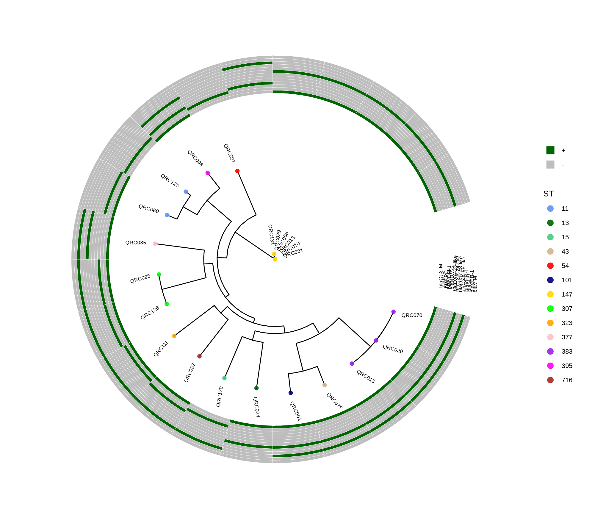
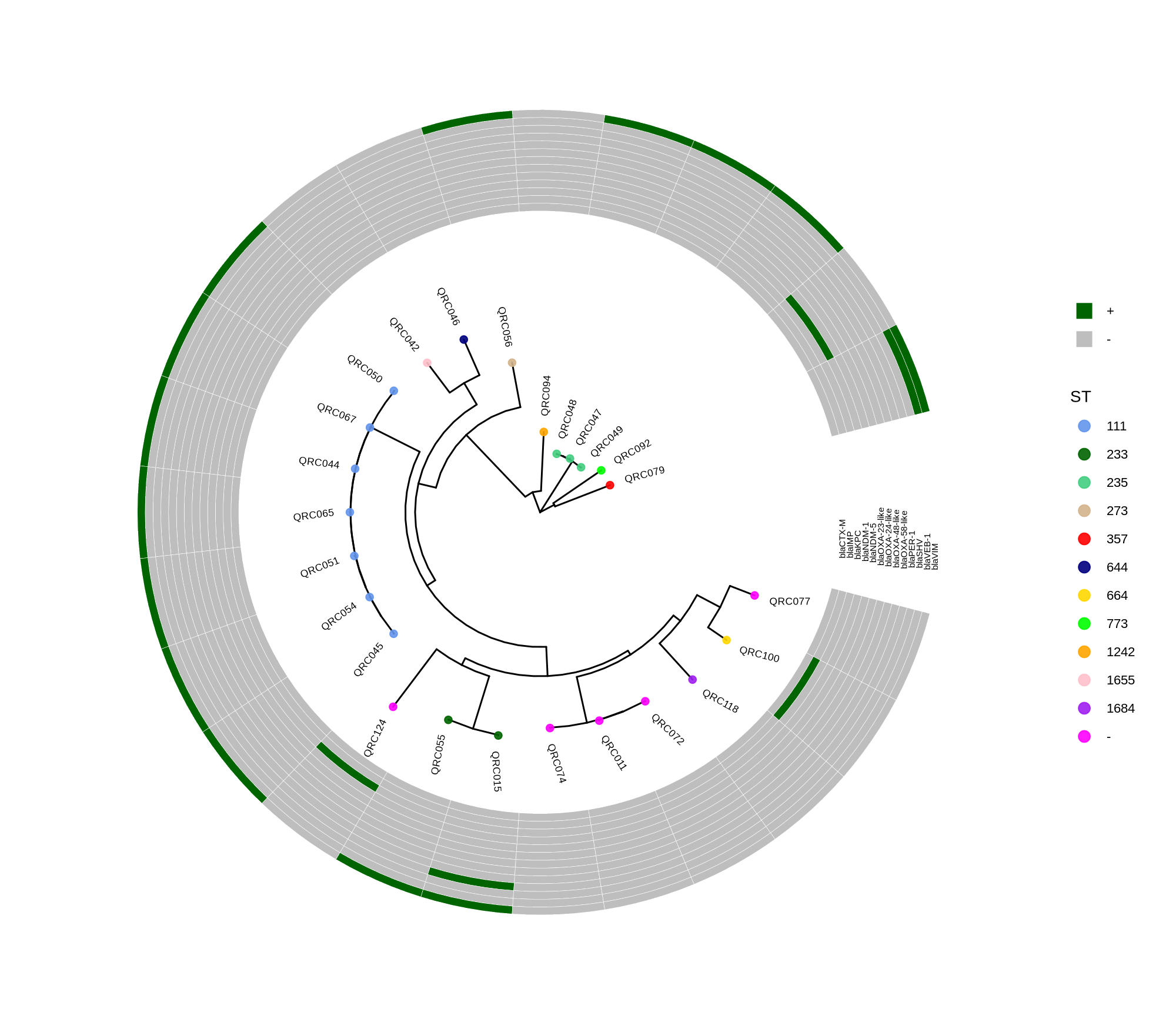
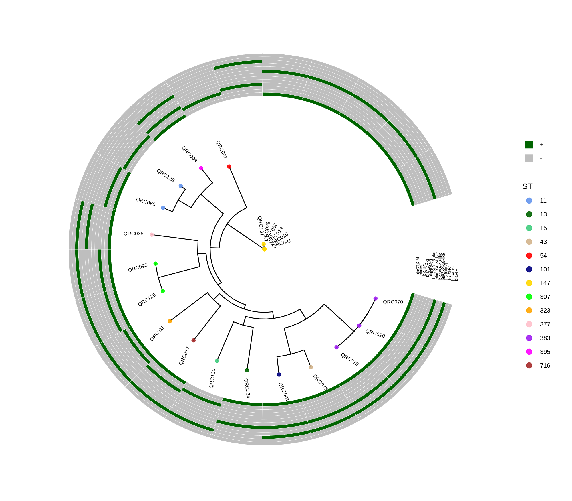
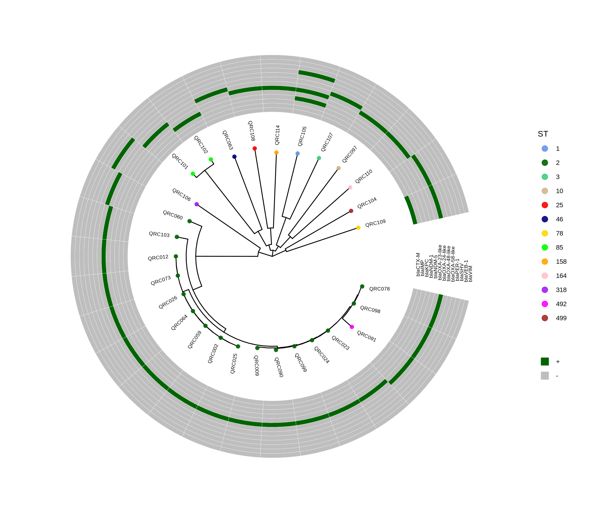
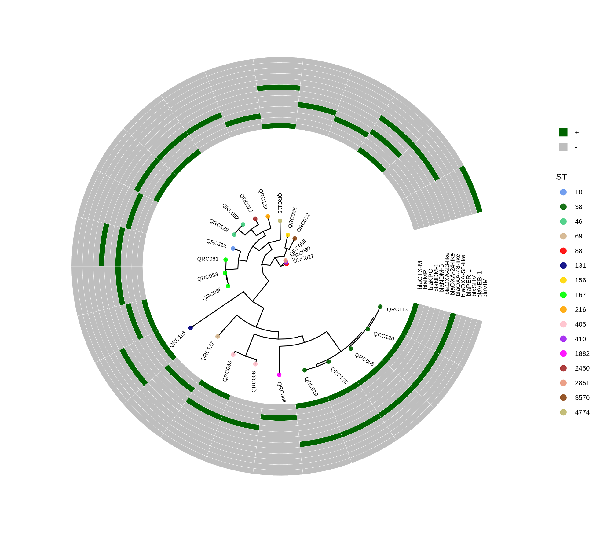
done

8. Visualization with ggtree and Heatmaps

Render circular core genome trees and overlay selected ARGs or gene presence/absence matrices.

Key R snippet:

library(ggtree)
library(ggplot2)
library(dplyr)
info <- read.csv("typing_until_ecpA.csv", sep="\t")
tree <- read.tree("raxml-ng/snippy.core.aln.raxml.tree")
p <- ggtree(tree, layout='circular', branch.length='none') %<+% info +
     geom_tippoint(aes(color=ST), size=4) + geom_tiplab2(aes(label=name), offset=1)
gheatmap(p, heatmapData2, width=4, colnames_angle=45, offset=4.2)

Output: multi‑layer circular tree (e.g., ggtree_and_gheatmap_selected_genes.png).


9. Final Analyses and Reporting

  • Compute pairwise SNP distances and identify potential clonal clusters using species‑specific thresholds (e.g., ≤17 SNPs for E. coli).
  • If clones exist, retain one representative per cluster for subsequent Boruta analysis or CA/EA metrics.
  • Integrate ARG heatmaps to the trees for intuitive visualization of resistance determinants relative to phylogeny.

Protocol Description Summary

This workflow systematically processes WGS data from multiple bacterial species:

  1. Annotation (Prokka) ensures consistent gene predictions.
  2. Pan‑genome alignment (Roary) captures core and accessory variation.
  3. Phylogenetic reconstruction (RAxML‑NG) provides species‑level evolutionary context.
  4. SNP‑distance computation (snp‑sites, snp‑dists) allows clonal determination and diversity quantification.
  5. Resistome analysis (Abricate, Diamond) characterizes antimicrobial resistance and virulence determinants.
  6. Visualization (ggtree + gheatmap) integrates tree topology with gene presence–absence or ARG annotations.

Properly documented, this end‑to‑end pipeline can serve as the Methods section for publication or as an online reproducible workflow guide.

Methods (for the manuscript). Genomes were annotated with PROKKA v1.14.5 [1]. A pangenome was built with Roary v3.13.0 [2] using default settings (95% protein identity) to derive a gene presence/absence matrix. Core genes—defined as present in 99–100% of isolates by Roary—were individually aligned with MAFFT v7 [3] and concatenated; the resulting multiple alignment was used to infer a maximum-likelihood phylogeny in RAxML-NG [4] under GTR+G, with 1,000 bootstrap replicates [5] and a random starting tree. Trees were visualized with the R package ggtree [6] in circular layout; tip colors denote sequence type (ST), with MLST assigned via PubMLST/BIGSdb [7]; concentric heatmap rings indicate the presence (+) or absence (-) of resistance genes.

  1. Seemann T. 2014. Prokka: rapid prokaryotic genome annotation. Bioinformatics 30:2068–2069.
  2. Page AJ, Cummins CA, Hunt M, Wong VK, Reuter S, Holden MTG, Fookes M, Falush D, Keane JA, Parkhill J. 2015. Roary: rapid large-scale prokaryote pan genome analysis. Bioinformatics 31:3691–3693.
  3. Katoh K, Standley DM. 2013. MAFFT multiple sequence alignment software version 7: improvements in performance and usability. Molecular Biology and Evolution 30:772–780.
  4. Kozlov AM, Darriba D, Flouri T, Morel B, Stamatakis A, Wren J. 2019. RAxML-NG: a fast, scalable and user-friendly tool for maximum likelihood phylogenetic inference. Bioinformatics 35:4453–4455.
  5. Felsenstein J. 1985. Confidence limits on phylogenies: an approach using the bootstrap. Evolution 39:783–791.
  6. Yu G, Smith DK, Zhu H, Guan Y, Lam TT-Y. 2017. ggtree: an R package for visualization and annotation of phylogenetic trees. Methods in Ecology and Evolution 8(1):28–36.
  7. Jolley KA, Bray JE, Maiden MCJ. 2018. Open-access bacterial population genomics: BIGSdb software, the PubMLST.org website and their applications. Wellcome Open Res 3:124.

Phylogenetic tree of E. coli isolates using the ggtree and ggplot2 packages (plotTreeHeatmap)

ggtree_and_gheatmap_ecoli
library(ggtree)
library(ggplot2)
library(dplyr)
#setwd("/home/jhuang/DATA/Data_Ben_Boruta_Analysis/plotTreeHeatmap_ecoli/")

info <- read.csv("isolate_ecoli_.csv", sep="\t", check.names = FALSE)
info$name <- info$Isolate
# make ST discrete
info$ST <- factor(info$ST)

tree <- read.tree("../ecoli_core_gene_tree_1000.raxml.bestTree")
cols <- c("10"="cornflowerblue","38"="darkgreen","46"="seagreen3","69"="tan","88"="red",  "131"="navyblue", "156"="gold",     "167"="green","216"="orange","405"="pink","410"="purple","1882"="magenta","2450"="brown", "2851"="darksalmon","3570"="chocolate4","4774"="darkkhaki")
# "290"="azure3", "297"="maroon","325"="lightgreen",     "454"="blue","487"="cyan", "558"="skyblue2", "766"="blueviolet"

#heatmapData2 <- info %>% select(Isolate, blaCTX.M, blaIMP, blaKPC, blaNDM.1, blaNDM.5, blaOXA.23.like, blaOXA.24.like, blaOXA.48.like, blaOXA.58.like, blaPER.1, blaSHV, blaVEB.1, blaVIM)  #ST,
heatmapData2 <- info %>% select(
    Isolate,
    `blaCTX-M`, blaIMP, blaKPC, `blaNDM-1`, `blaNDM-5`,
    `blaOXA-23-like`, `blaOXA-24-like`, `blaOXA-48-like`, `blaOXA-58-like`,
    `blaPER-1`, blaSHV, `blaVEB-1`, blaVIM
)
rn <- heatmapData2$Isolate
heatmapData2$Isolate <- NULL
heatmapData2 <- as.data.frame(sapply(heatmapData2, as.character))
rownames(heatmapData2) <- rn

#heatmap.colours <- c("darkred", "darkblue", "darkgreen", "grey")
#names(heatmap.colours) <- c("MT880870","MT880871","MT880872","-")

#heatmap.colours <- c("cornflowerblue","darkgreen","seagreen3","tan","red",  "navyblue", "gold",     "green","orange","pink","purple","magenta","brown", "darksalmon","chocolate4","darkkhaki", "azure3", "maroon","lightgreen",     "blue","cyan", "skyblue2", "blueviolet",       "darkred", "darkblue", "darkgreen", "grey")
#names(heatmap.colours) <- c("2","5","7","9","14", "17","23",   "35","59","73", "81","86","87","89","130","190","290", "297","325",    "454","487","558","766",       "MT880870","MT880871","MT880872","-")

#heatmap.colours <- c("cornflowerblue","darkgreen","seagreen3","tan","red",  "navyblue", "purple",     "green","cyan",       "darkred", "darkblue", "darkgreen", "grey",  "darkgreen", "grey")
#names(heatmap.colours) <- c("SCCmec_type_II(2A)", "SCCmec_type_III(3A)", "SCCmec_type_III(3A) and SCCmec_type_VIII(4A)", "SCCmec_type_IV(2B)", "SCCmec_type_IV(2B&5)", "SCCmec_type_IV(2B) and SCCmec_type_VI(4B)", "SCCmec_type_IVa(2B)", "SCCmec_type_IVb(2B)", "SCCmec_type_IVg(2B)",  "I", "II", "III", "none", "+","-")

heatmap.colours <- c("darkgreen", "grey")
names(heatmap.colours) <- c("+","-")

#mydat$Regulation <- factor(mydat$Regulation, levels=c("up","down"))
#circular

p <- ggtree(tree, layout='circular', branch.length='none') %<+% info + geom_tippoint(aes(color=ST)) + scale_color_manual(values=cols) + geom_tiplab2(aes(label=name), offset=1)
png("ggtree.png", width=1260, height=1260)
#svg("ggtree.svg", width=1260, height=1260)
p
dev.off()

#gheatmap(p, heatmapData2, width=0.1, colnames_position="top", colnames_angle=90, colnames_offset_y = 0.1, hjust=0.5, font.size=4, offset = 5) + scale_fill_manual(values=heatmap.colours) +  theme(legend.text = element_text(size = 14)) + theme(legend.title = element_text(size = 14)) + guides(fill=guide_legend(title=""), color = guide_legend(override.aes = list(size = 5)))

png("ggtree_and_gheatmap_mibi_selected_genes.png", width=1590, height=1300)
#svg("ggtree_and_gheatmap_mibi_selected_genes.svg", width=17, height=15)
gheatmap(p, heatmapData2, width=2, colnames_position="top", colnames_angle=90, colnames_offset_y = 2.0, hjust=0.7, font.size=4, offset = 8) + scale_fill_manual(values=heatmap.colours) +  theme(legend.text = element_text(size = 16)) + theme(legend.title = element_text(size = 16)) + guides(fill=guide_legend(title=""), color = guide_legend(override.aes = list(size = 5)))
dev.off()

# ---------

# 1) Optional: shrink tree to create more outer space (keeps relative scale)
tree_small <- tree
tree_small$edge.length <- tree_small$edge.length * 0.4    # try 0.3–0.5

# 2) Height after shrinking
ht <- max(ape::node.depth.edgelength(tree_small))

# 3) Base tree
info$ST <- factor(info$ST)
p <- ggtree(tree_small, layout = "circular", open.angle = 20) %<+% info +
    geom_tippoint(aes(color = ST), size = 1.4) +
    geom_tiplab2(aes(label = name), size = 1.4, offset = 0.02 * ht) +
    scale_color_manual(values = cols)

# 4) Reserve room outside the tips
off <- 0.30 * ht   # gap
wid <- 2.80 * ht   # ring thickness
mar <- 0.25 * ht
p_wide <- p + xlim(0, ht + off + wid + mar)

# 5) Ensure discrete values are factors and keep both levels
heatmapData2[] <- lapply(heatmapData2, function(x) factor(x, levels = c("+","-")))

# 6) Draw the heatmap
png("ggtree_and_gheatmap_readable.png", width = 3600, height = 3200, res = 350)
gheatmap(
    p_wide, heatmapData2,
    offset = off,
    width  = wid,
    color  = "white",            # borders between tiles
    colnames = TRUE,
    colnames_position = "top",
    colnames_angle = 0,
    colnames_offset_y = 0.04 * ht,
    hjust = 0.5,
    font.size = 7
) +
    scale_fill_manual(values = c("+"="darkgreen", "-"="grey"), drop = FALSE) +
    guides(
        fill  = guide_legend(title = "", override.aes = list(size = 4)),
        color = guide_legend(override.aes = list(size = 3))
    )
dev.off()

#-------------- plot with true scale -------------

# tree height (root → farthest tip)
ht <- max(ape::node.depth.edgelength(tree))

# circular tree with a small opening and compact labels
p <- ggtree(tree, layout = "circular", open.angle = 20) %<+% info +
    geom_tippoint(aes(color = ST), size = 1.8, alpha = 0.9) +
    geom_tiplab2(aes(label = name), size = 2.2, offset = 0.06 * ht) +
    scale_color_manual(values = cols) +
    theme(legend.title = element_text(size = 12),
                legend.text  = element_text(size = 10))

# higher-DPI export so small cells look crisp
png("ggtree_true_scale.png", width = 2400, height = 2400, res = 300)
p
dev.off()

# --- Heatmap: push it further out and make it wider ---
#svg("ggtree_and_gheatmap_mibi_selected_genes_true_scale.svg",
#    width = 32, height = 28)

png("ggtree_and_gheatmap_mibi_selected_genes_true_scale.png",
        width = 2000, height = 1750,  res = 200)

gheatmap(
    p, heatmapData2,
    offset = 0.24 * ht,         # farther from tips (was 0.08*ht)
    width  = 20.0 * ht,         # much wider ring (was 0.35*ht)
    color  = "white",           # thin tile borders help readability
    colnames_position  = "top",
    colnames_angle     = 90,     # keep column labels horizontal to save space
    colnames_offset_y  = 0.08 * ht,
    hjust = 0.1,
    font.size = 2.6               # bigger column label font
) +
    scale_fill_manual(values = heatmap.colours) +
    guides(fill  = guide_legend(title = "", override.aes = list(size = 4)),
                 color = guide_legend(override.aes = list(size = 3))) +
    theme(legend.position = "right",
                legend.title    = element_text(size = 10),
                legend.text     = element_text(size = 8))
dev.off()

This R script visualizes a phylogenetic tree of E. coli isolates using the ggtree and ggplot2 packages, annotated with sequence type (ST) colors and a heatmap showing the presence or absence of antimicrobial resistance genes. It creates several versions of the circular tree figure to adjust scaling and readability.

Key Steps

  1. Load libraries and data The code imports ggtree, ggplot2, and dplyr, reads isolate metadata (isolate_ecoli_.csv), and loads a phylogenetic tree file (ecoli_core_gene_tree_1000.raxml.bestTree).12
  2. Prepare metadata It defines each isolate’s name and converts the sequence type (ST) into a categorical factor. A subset of columns (various bla resistance gene markers) is selected to create a heatmap data matrix, where each gene’s presence (“+”) or absence (“–”) will be visualized.
  3. Define color schemes Different STs are assigned distinct colors, and binary gene presence/absence states (“+”, “–”) mapped to “darkgreen” and “grey,” respectively.3
  4. Plot tree with annotation The main tree is plotted circularly using:
p <- ggtree(tree, layout='circular', branch.length='none') %<+% info + 
     geom_tippoint(aes(color=ST)) + scale_color_manual(values=cols)

Tip labels are added for isolates, and STs are colored as per the legend.

  1. Add heatmap (gene presence/absence) The gheatmap() function appends the gene matrix to the tree, aligning rows with the tree tips and providing a heatmap of resistance gene patterns.23
  2. Export figures Multiple PNGs are generated:
    • ggtree.png: Basic circular tree
    • ggtree_and_gheatmap_mibi_selected_genes.png: Tree + resistance gene heatmap
    • Scaled versions with adjusted offsets and spacing for improved readability and “true-scale” representations

Final Output

The resulting figures show a circular phylogenetic tree annotated by ST colors, accompanied by a ring-style heatmap indicating the distribution of key resistance genes across isolates. The layout adjustments (tree shrinking, offset tuning, width scaling) ensure legibility when genes or isolates are numerous.23 4567891011121314151617181920

雙側足底筋膜炎與體外衝擊波治療(ESWT)全指南

概述

雙側足底筋膜炎是成人足跟痛最常見的原因之一,典型表現為清晨或久坐後首次下地時足跟內側刺痛,走動少許可緩解,但久站久走或跑步後又加重。212223 病因多與足底筋膜反覆牽拉導致的微撕裂與退行性改變相關,而非單純的急性發炎,雙側受累時步態代償更明顯、承重耐受度下降。242526

定義與病理

雖名為“炎”,但顯微與臨床更多呈現著骨點病變與退行性改變(微撕裂、膠原退變),而非典型急性炎細胞浸潤。24 病灶多起於跟骨內側結節的足底筋膜近端附著點,可見筋膜增厚與壓痛;影像可能出現跟骨骨刺,但骨刺本身並非疼痛直接原因。252724 足底筋膜自跟骨延伸至足趾底部,負責支撐足弓並吸收衝擊,因此在跑跳或久站等反覆負荷下容易受損。2321

常見症狀

足跟內側或足弓處的銳痛/刺痛,清晨首步痛最明顯,稍活動後可暫時減輕,但長時間負重後再度加重。2621 雙側病例中,兩足承重對稱受限,代償步態更突出,影響長時間站立與行走的耐受度。2624

危險因素

  • 足弓異常(扁平足或高弓足)與力線偏差會增加筋膜應力。272524
  • 腓腸肌/比目魚肌緊張與跟腱緊繃導致踝關節背屈受限。2524
  • 久站、跳躍、長距離或下坡跑,以及突然提高訓練量與硬地面負荷。242526
  • 體重增加/肥胖與足跟脂肪墊退變、不合適鞋履(支撐或緩衝不足)。252624
  • 雙側受累常提示雙足共同的生物力學與負荷模式問題,需要對稱化處理。2624

診斷要點

臨床診斷以病史與查體為主:跟骨前內側足底壓痛、清晨首步痛、踝背屈受限並結合危險因素評估。2125 必要時超音波可見筋膜增厚與水腫,X光可見跟骨骨刺並協助排除應力性骨折等其他病變。25

保守治療

多數患者在非手術治療下於數月內改善,治療目標為鎮痛、恢復筋膜與小腿後群柔韌性、優化足弓力線與支撐,並逐步回歸活動(雙足同步管理)。2325

  • 負荷管理:減少高衝擊與久站,分段活動,循序漸進增加訓練量(雙足均衡)。2426
  • 冰敷與短期口服NSAIDs依醫囑鎮痛。2325
  • 拉伸訓練:足底筋膜特異性拉伸與小腿後群(腓腸肌/比目魚肌)拉伸,每日多次、逐步加量。2325
  • 夜間足托維持中立至輕度背屈位,以減輕晨起首步痛。2523
  • 矯形支撐:足弓鞋墊、足跟杯/墊,必要時貼紮短期矯正力線。2325
  • 物理治療:本體感覺與肌力訓練、軟組織鬆解,必要時超音波等,依個體化評估執行。2825

體外衝擊波治療(ESWT)

ESWT (Extrakorporale Stoßwellentherapie) 為非侵入性療法,透過短時高壓聲學衝擊刺激組織修復並達到鎮痛,常於保守治療無效的慢性病例採用,臨床上常規劃約三次為一組的門診療程。2425 模式與定位:分為聚焦型(fESWT)與徑向型(rESWT),於最痛點經皮定位施打,單次治療僅需數分鐘,可在無麻醉下完成。2425 療效與節奏:目標為中長期減痛與功能提升,常在數週至數月逐步改善;並行拉伸、鞋墊與負荷管理可提高療效與持久性。2523 不良反應:多為短暫壓痛、紅腫或小淤斑,嚴重併發症罕見,整體安全性良好。2425

其他可選方案

超音波導引下糖皮質激素注射可提供短期鎮痛,但存在復發與筋膜損傷風險,須審慎權衡;對於頑固疼痛,衝擊波治療可作為進一步的非侵入選擇。2524 針灸在4–8週內的止痛有一定證據,但長期優勢未確立,宜與標準療法綜合評估。29 手術(如部分筋膜鬆解)僅限於長期頑固且保守療法失敗者,比例相當低。24

預後與復發

大多數患者在規範保守治療下於數月內明顯改善,部分病例一年內可自限;然而疼痛可能反覆,需長期維持拉伸與力線管理。2524 雙側病變因整體負荷更高、代償更多,康復節奏宜更循序,並強化小腿後群柔韌性與足弓支撐。2324

日常建議

  • 選擇具良好足弓支撐與後跟緩衝的鞋款,及時更換磨損鞋底,避免硬地赤足久走。2325
  • 循序遞增運動量,交替低衝擊訓練(如騎行/游泳),並做好體重管理以減輕足跟負荷。2625
  • 每日2–3次進行足底筋膜與小腿後群拉伸,每次保持20–30秒,重複3–5組。2325
  • 晨起下地前先做踝泵與毛巾拉伸,減少首步痛;需久站工作者可採用軟墊與分段休息策略。2523
  • 若持續數週無改善或出現夜間靜息痛、神經症狀,應就醫評估以排除其他病因。25 3031323334353637

RNA-seq + Proteomics Integration Workflow (Δsbp; MH & TSB)

cd results/star_salmon/degenes

The article uses the following Python scripts (please see Data_Michelle_RNAseq_2025_scripts.zip).

* map_orf_1to1_progress_safe.py
* map_orf_1to1_progress.py (deprecated)
* check_missing_uniprot_fastas.py
* rescue_missing_uniprot.py
* compare_transcript_protein.py
* make_rna_only_present_excels.py (needs debugging)
* make_rna_only_not_in_protDE.py (needs debugging)
* map_symbols.py (deprecated)

0) Goal

  • Match IDs: convert UniProt protein IDs to gene symbols to allow direct comparison with RNA-seq.
  • Merge datasets by gene_symbol and retain: protein_log2FC, protein_padj, rna_log2FC, rna_padj.
  • Classify each gene/protein into:
    • both_significant_same_direction
    • both_significant_opposite_direction
    • protein_only_significant
    • rna_only_significant
  • Subset analysis: examine proteins significant in proteomics but not in RNA-seq (and vice versa) to identify post-transcriptional regulation, stability, secretion/export, or translational effects.

Comparisons (process first: 1–6)

MH medium

Index Comparison (normalized) RNA-seq Proteomics
1 Δsbp_2h_vs_WT_2h (alt. Δsbp_1h_vs_WT_1h)
2 Δsbp_4h_vs_WT_4h
3 Δsbp_18h_vs_WT_18h

TSB medium

Index Comparison (normalized) RNA-seq Proteomics
4 Δsbp_2h_vs_WT_2h (alt. Δsbp_1h_vs_WT_1h)
5 Δsbp_4h_vs_WT_4h
6 Δsbp_18h_vs_WT_18h
7 Δsbp_1h_vs_Δsbp_4h
8 Δsbp_4h_vs_Δsbp_18h
9 WT_1h_vs_WT_4h
10 WT_4h_vs_WT_18h

1) Environment

mamba activate rnaseq_prot_comparison
mamba install -c conda-forge biopython pandas openpyxl requests requests-cache tqdm -y
mamba activate rnaseq_prot_comparison

2) Populate cache once (per‑ID fetch via aligner)

# MH (example outcome: mapped 589)
python map_orf_1to1_progress_safe.py \
  --rna_fa ../../genome/genome.transcripts.fa \
  --prot_xlsx Aug25_AG_Rohde_Order_609_Michelle-MH-Medium-abgekratzer-Biofilm.xlsx \
  --prot_kind mh \
  --min_aa 10 \
  --requests_cache \
  --out map_mh.csv

# Expected console example:
# ORFs translated: 2319; proteins: 616; mapped: 589
# Output: map_mh.csv

3) Check which UniProt IDs are missing (cache and stream)

python check_missing_uniprot_fastas.py \
  --mh_xlsx "Aug25_AG_Rohde_Order_609_Michelle-MH-Medium-abgekratzer-Biofilm.xlsx" \
  --tsb_xlsx "250618_Report_AG_Rohde_Michelle_Savickis_BS_ND-schalen-zeitreihe-TSB-Medium.xlsx" \
  --cache cache/uniprot_fastas \
  --out check_report.txt

# Example:
# Total unique accessions: 1781
# In cache (non-empty FASTA): 1296
# Missing in cache: 485
# Present via UniProt stream now: 0
# Missing via UniProt stream now: 1781

4) Rescue missing accessions (UniSave → UniParc → UniProtKB remap)

  • After each run, check rescue_summary.txt and rerun the checker before redoing alignments.
# 4.1) Rescue cache-missing
python rescue_missing_uniprot.py --miss_file missing_cache.txt --cache cache/uniprot_fastas

# 4.2) Re-check
python check_missing_uniprot_fastas.py \
  --mh_xlsx "Aug25_AG_Rohde_Order_609_Michelle-MH-Medium-abgekratzer-Biofilm.xlsx" \
  --tsb_xlsx "250618_Report_AG_Rohde_Michelle_Savickis_BS_ND-schalen-zeitreihe-TSB-Medium.xlsx" \
  --cache cache/uniprot_fastas \
  --out check_report_after_rescue.txt

# Example (OK to proceed):
# Total unique accessions: 1781
# In cache (non-empty FASTA): 1781
# Missing in cache: 0
# Present via UniProt stream now: 0
# Missing via UniProt stream now: 1781

# 4.3) Optional: rescue stream-missing
python rescue_missing_uniprot.py --miss_file missing_stream.txt --cache cache/uniprot_fastas

Notes:

  • If “Present via UniProt stream now” is 0, it usually indicates a streaming query/parse/limit issue; cached per‑accession FASTAs are valid and sufficient for alignment.

5) Rerun the aligner with rescued FASTAs

# MH final
python map_orf_1to1_progress_safe.py \
  --rna_fa ../../genome/genome.transcripts.fa \
  --prot_xlsx Aug25_AG_Rohde_Order_609_Michelle-MH-Medium-abgekratzer-Biofilm.xlsx \
  --prot_kind mh \
  --min_aa 10 \
  --requests_cache \
  --out map_mh_final.csv

# TSB (cache already populated; re-run if desired)
python map_orf_1to1_progress_safe.py \
  --rna_fa ../../genome/genome.transcripts.fa \
  --prot_xlsx 250618_Report_AG_Rohde_Michelle_Savickis_BS_ND-schalen-zeitreihe-TSB-Medium.xlsx \
  --prot_kind tsb \
  --min_aa 10 \
  --requests_cache \
  --out map_tsb.csv

6) Final comparison (merge, classify, export)

# Build merged comparisons (1–6), classify categories
python compare_transcript_protein.py \
  --map_mh map_mh_final.csv \
  --map_tsb map_tsb.csv \
  --out_dir results_compare \
  --alpha 0.05

# Convert CSVs to a single Excel workbook
~/Tools/csv2xls-0.4/csv_to_xls.py \
  summary_counts.csv MH_2h_merged.csv MH_4h_merged.csv MH_18h_merged.csv \
  TSB_2h_merged.csv TSB_4h_merged.csv TSB_18h_merged.csv \
  -d',' -o RNAseq-Proteomics_deltasbp_MH-TSB_2h4h18h_summary_20251002.xlsx

# Optional: export RNA-only-present genes per comparison (empty proteomics fields)
python make_rna_only_present_excels.py --out_dir rna_only_present_excels

7) Why counts differ (e.g., 1173(1319) vs 1107; TSB 663 vs 650)

  • The aligner uses “unique, usable” FASTA sequences; duplicates, deprecated/secondary or invalid accessions, and empty/invalid sequences are filtered, so usable proteins can be fewer than attempted fetches.
  • TSB 663 vs 650: about 13 entries typically drop due to duplicate/merged IDs, obsolete accessions, decoy/contaminant-like strings, or missing gene symbols that prevent a 1‑to‑1 map with RNA-seq.

中文备注: 结论:对齐阶段用的是“可用且唯一”的蛋白序列集合,因此数量会小于最初尝试获取的条目数;对 TSB,663 行在规范化与去重后得到 650 个可用记录属正常现象。


8) Report (email-ready text)

As mentioned, the IDs between proteomics and RNA‑seq were matched based on direct sequence alignment (ORF nucleotide sequences translated and aligned to UniProt protein FASTA) to ensure 1‑to‑1 mapping and unambiguous ID correspondence.

Please note that the recorded counts are constrained by the proteomics differentially expressed (DE) tables: for MH medium, 1107 proteins/genes; for TSB medium, 650. The RNA‑seq DE lists are larger overall, but the integration and comparisons are based on entities present in both proteomics and RNA‑seq.

For the overlap between the two datasets, each gene/protein was placed into one of five categories:

  • not_significant_in_either
  • rna_only_significant
  • protein_only_significant
  • both_significant_same_direction
  • both_significant_opposite_direction

The attached Excel file contains per‑comparison merged tables (protein_log2FC, protein_padj, rna_log2FC, rna_padj), category calls for each entry, and summary counts for quick review.


9) Notes \& assumptions

  • MH comparison blocks are read in 18h, 4h, 1h order from Ord_609 (three repeated “Log2 difference / q-value (Benjamini FDR)” blocks after intensities). If the template differs, adjust the mapping.
  • TSB comparisons are explicitly labeled (sbp vs Control at 1h/4h/18h) and are used verbatim.
  • Gene symbol preference: use proteomics-provided symbols (MH via GN=; TSB via Gene Symbol); otherwise fall back to RNA Preferred_name by locus to unify merge keys.
  • Significance: default padj < 0.05 for both datasets (set via –alpha). Add effect-size filters if needed.

10) TODOs

  • Cluster by presence across platforms: using TSB 650 and MH 1319 proteins, derive 5+1 groups; the +1 group contains genes not occurring in the proteomics results; Namely, RNA-only-present category: implemented—prefer set-difference on gene_symbol (RNA DE minus proteomics DE) per comparison to produce concise lists and avoid many‑to‑many expansions.
  • Re-run proteomics DE with Gunnar’s project scripts to expand DE coverage if needed.

Appendix: Deprecated symbol-only mapping (for reference)

# (Deprecated) Symbol-based mapping reached ~35% overlap → switched to sequence-alignment-based mapping.

python map_symbols.py \
  --rna DEG_Annotations_deltasbp_MH_4h_vs_WT_MH_4h-all.xlsx \
  --prot Aug25_AG_Rohde_Order_609_Michelle-MH-Medium-abgekratzer-Biofilm.xlsx \
  --prot_kind mh

# RNA rows total: 2344
# RNA symbols:    1460
# Proteomics symbols: 1280
# Intersect (symbols): 519
# Coverage vs RNA symbols:        35.5%
# Coverage vs Proteomics symbols:  40.5%
# Coverage vs all RNA rows:        22.1%

python map_symbols.py \
  --rna DEG_Annotations_deltasbp_MH_2h_vs_WT_MH_2h-all.xlsx \
  --prot 250618_Report_AG_Rohde_Michelle_Savickis_BS_ND-schalen-zeitreihe-TSB-Medium.xlsx \
  --prot_kind tsb

# RNA rows total: 2344
# RNA symbols:    1460
# Proteomics symbols: 568
# Intersect (symbols): 512
# Coverage vs RNA symbols:        35.1%
# Coverage vs Proteomics symbols:  90.1%
# Coverage vs all RNA rows:        21.8%

38394041424344454647