Single-Molecule Binding/Bleaching Detection Pipeline for Data_Vero_Kymographs

“What is confirmed is hexamer and double-hexamer binding to DNA, whereas monomer/dimer binding to DNA is not confirmed.”

Overview

This workflow robustly detects and quantifies molecular binding and bleaching events from single-molecule fluorescence trajectories. It employs Hidden Markov Model (HMM) analysis to convert noisy intensity data into interpretable discrete state transitions, using a combination of MATLAB/Octave and Python scripts.

Step 1: ICON HMM Fitting per Track

Runs icon_from_track_csv.m, loading each track’s photon count data, fitting a HMM (via the ICON algorithm), and saving results (icon_analysis_track_XX.mat).
Key outputs:
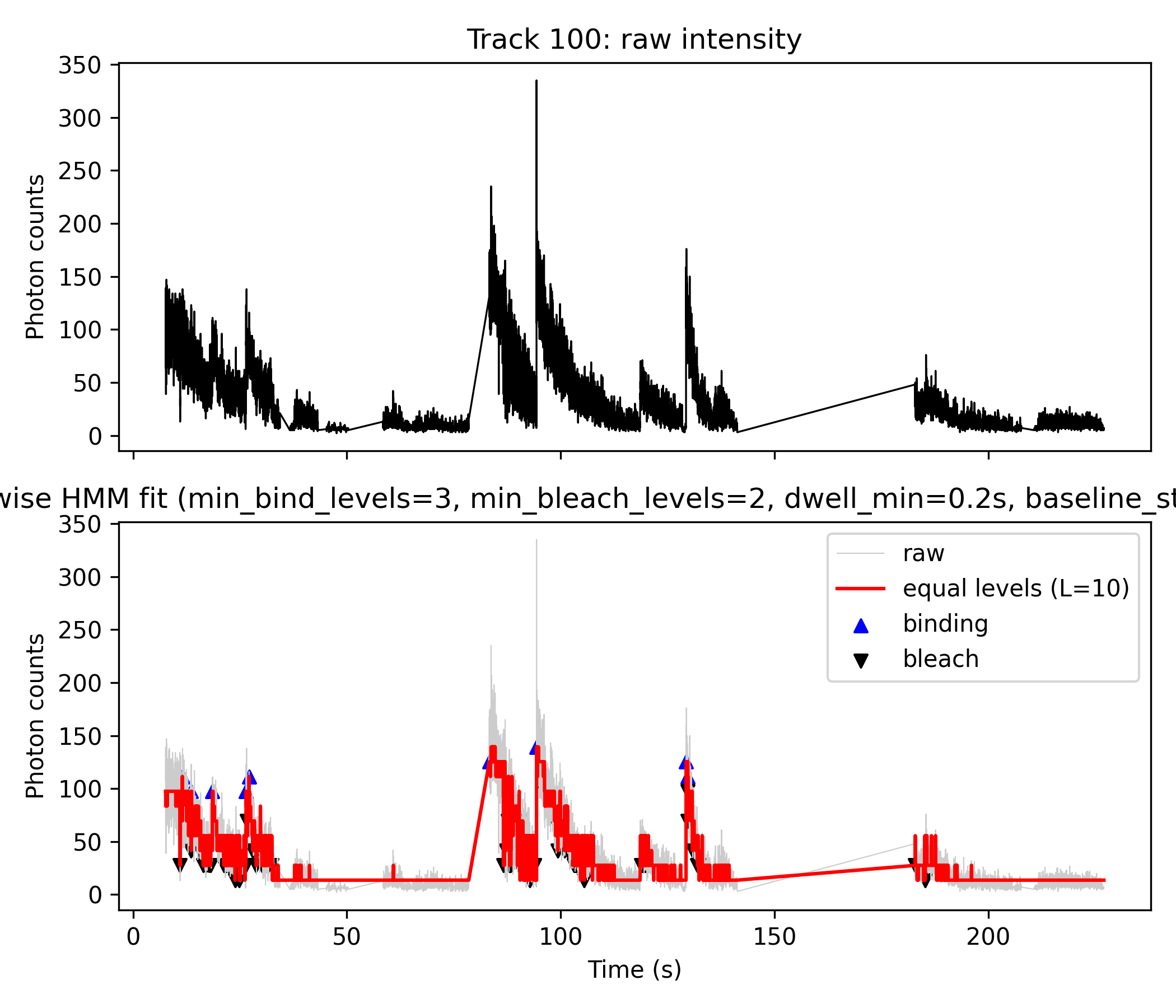
- Raw time series × photon counts (used for the black curve in plot, top and background of bottom plot)
- HMM mean state sequence (m_mod)
Example command:

for track_id in 0 1 2 3 4 5 6 7 8 9 10 11 12 13 14; do
  octave icon_post_equal_levels.m icon_analysis_track_${track_id}.mat
done

Step 2: Discretize HMM Means (Not Used for Plot Generation)

(Optional) Runs icon_post_equal_levels.m to generate equal_levels_track_XX.mat, which contains a stepwise, discretized version of the HMM fit.
This step is designed for diagnostic parameter tuning (finding L_best), but the plotting script does not use these files for figure generation.

后处理成“等间距台阶 + bleaching step” (这些文件主要用来“告诉你 L 选多少比较合适”(namely L_best)，而不是直接给 Python 画图用).

for track_id in 0 1 2 3 4 5 6 7 8 9 10 11 12 13 14; do
octave icon_post_equal_levels.m icon_analysis_track_${track_id}.mat
done
# 生成 equal_levels_track_100.mat for Step 4

Step 3: Event Detection \& Visualization (Python)

Core script: plot_fig4AB_python.py
Loads icon_analysis_track_XX_matlab.mat produced by Step 1.
Black plot (top and gray in lower panel): Raw photon count data.
Red plot (lower panel): Stepwise HMM fit — generated by mapping the HMM mean trajectory to L (e.g. 10) equally spaced photon count levels (L_best).
Event detection:
- Blue triangles: Up-step events (binding)
- Black triangles: Down-step events (bleaching)
- Uses in-script logic to detect transitions meeting user-set thresholds:
  - min_levels_bind=3, min_levels_bleach=2, dwell_min=0.2s, baseline_state_max=5
- Produces both plots and machine-readable event tables (CSV, Excel)
Sample commands:

mamba activate kymo_plots
for track_id in 0 1 2 3 4 5 6 7 8 9 10 11 12 13 14 100; do
  python plot_fig4AB_python.py ${track_id} 10 3 2 0.2 5
done

Step 4: (For Future) Aggregation

icon_multimer_histogram.m is prepared for future use to aggregate results from many tracks (e.g., make multimer/stoichiometry histograms).
This step is not used for the current plots.

octave icon_multimer_histogram.m
# for subset use:
octave icon_multimer_histogram.m "equal_levels_track_1*.mat"
#→ 得到 multimer_histogram.png, 就是你的 Fig. 4C-like 图.

Figure Explanation (e.g. Track 14 and Track 100)

Top panel (black line): Raw photon counts (z).
- Direct output from Step 1 HMM analysis; visualizes the original noisy fluorescence trace.
Bottom panel:
- Gray line: Raw photon counts for direct comparison.
- Red line: Step-wise fit produced by discretizing the HMM mean (m_mod) from Step 1 directly inside the python script.
- Blue “▲”: Detected binding (upward) events.
- Black “▼”: Detected bleaching (downward) events.
Event Table: Both “binding” and “bleach” events are exported with details: time, photon count, state transition, and dwell time.

Note:

For these figures, only Step 1 and Step 3 are used.
Step 2 is for diagnostic/discretization, but in our current pipeline, L_best was given directly with 10, was not calculated from Step 2, therefore Step 2 was not used.
Step 4 is left for future population summaries.

Key Script Function Descriptions

1. icon_from_track_csv.m (Octave/MATLAB)

Loads a csv photon count time sequence for a single molecule track.
Infers hidden states and mean trajectory with ICON/HMM.
Saves all variables for python to use.

2. plot_fig4AB_python.py (Python)

Loads .mat results: time (t), photons (z), and HMM means (m_mod).
Discretizes the mean trajectory into L equal steps, maps continuous states to nearest discrete, and fits photon counts by linear regression for step heights.
Detects step transitions corresponding to binding or bleaching based on user parameters (size thresholds, dwell filters).
Plots raw data + stepwise fit, annotates events, and saves tables.

(Script excerpt, see full file for details):

def assign_to_levels(m_mod, levels):
    # Map every m_mod value to the nearest discrete level
    ...

def detect_binding_bleach_from_state(...):
    # Identify up/down steps using given jump sizes and baseline cutoff
    ...

def filter_short_episodes_by_dwell(...):
    # Filter events with insufficient dwell time
    ...
...
if __name__ == "__main__":
    # Parse command line args, load .mat, process and plot

Complete Scripts

See attached files for full script code:

icon_from_track_csv.m
plot_fig4AB_python.py
icon_post_equal_levels.m (diagnostic, not used for current figures)
icon_multimer_histogram.m (future)

Example Event Table Output

The python script automatically produces a CSV/Excel file summarizing:

Event type (“binding” or “bleach”)
Time (seconds)
Photon count (at event)
States before/after the event
Dwell time (for binding)

In summary:

Figures output from plot_fig4AB_python.py directly visualize both binding and bleaching events as blue (▲) and black (▼) markers, using logic based on HMM analysis and transition detection within the Python code, without any direct dependence on Step 2 “equal_levels” files. This approach is both robust and reproducible for detailed single-molecule state analysis. [^1][^2]

⁂

icon_from_track_csv.m

clear all;
%% icon_from_track_csv.m
%% 用 ICON HMM 分析你自己的 track_intensity CSV 数据
%%
%% 用法（命令行）：
%%   octave icon_from_track_csv.m your_track_intensity_file.csv [track_id]
%%
%% - your_track_intensity_file.csv:
%%     3 列分号分隔：
%%     # track index;time (seconds);track intensity (photon counts)
%% - track_id（可选）:
%%     要分析的 track_index 数值，例如 0、2、10、100 等
%%     如果不给，则自动：
%%       - 若存在 track 100，则用 100
%%       - 否则用第一个 track

%%--------------------------------------------
%% 0. 处理命令行参数
%%--------------------------------------------
arg_list = argv();
if numel(arg_list) < 1
    error("Usage: octave icon_from_track_csv.m 
<track_intensity_csv> [track_id]");
end

input_file = arg_list{1};
track_id_arg = NaN;
if numel(arg_list) >= 2
    track_id_arg = str2double(arg_list{2});
end

fprintf("Input CSV : %s\n", input_file);
if ~isnan(track_id_arg)
    fprintf("Requested track_id: %g\n", track_id_arg);
end

%% 链接 ICON sampler 的源码
%addpath('sampler_SRC');

% 尝试加载 statistics 包（gamrnd 在这里）
try
    pkg load statistics;
catch
    warning("Could not load 'statistics' package. Please install it via 'pkg install -forge statistics'.");
end

%%--------------------------------------------
%% 1. 读入 3 列 CSV: track_index;time;counts
%%--------------------------------------------
fid = fopen(input_file, 'r');
if fid < 0
    error("Cannot open file: %s", input_file);
end

% 第一行是注释头 "# track index;time (seconds);track intensity (photon counts)"
header_line = fgetl(fid);  %#ok
<NASGU>

% 后面每行: track_index;time_sec;intensity
data = textscan(fid, "%f%f%f", "Delimiter", ";");
fclose(fid);

track_idx = data{1};
time_sec  = data{2};
counts    = data{3};

% 按 track 和时间排序，保证序列有序
[~, order] = sortrows([track_idx, time_sec], [1, 2]);
track_idx = track_idx(order);
time_sec  = time_sec(order);
counts    = counts(order);

tracks = unique(track_idx);
fprintf("Found %d tracks: ", numel(tracks));
fprintf("%g ", tracks);
fprintf("\n");

%%--------------------------------------------
%% 2. 选择要分析的 track
%%--------------------------------------------
if ~isnan(track_id_arg)
    tr = track_id_arg;
else
    % 如果存在 track 100，则优先选 100（你自己定义的 accumulated 轨迹）
    if any(tracks == 100)
        tr = 100;
    else
        tr = tracks(1);   % 否则就选第一个
    end
end

if ~any(tracks == tr)
    error("Requested track_id = %g not found in file.", tr);
end

fprintf("Using track_id = %g for ICON analysis.\n", tr);

sel = (track_idx == tr);
t   = time_sec(sel);
z   = counts(sel);

% 按时间排序（理论上已经排过一次，这里再保险）
[ t, order_t ] = sort(t);
z = z(order_t);

z = z(:);  % 列向量
N = numel(z);
fprintf("Track %g has %d time points.\n", tr, N);

%%--------------------------------------------
%% 3. 设置 ICON 参数（与原始脚本一致）
%%--------------------------------------------

% 浓度（Dirichlet 相关超参数）
opts.a = 1;   % Transitions (alpha)
opts.g = 1;   % Base (gamma)

% 超参数 Q
opts.Q(1) = mean(z);         % mean of means (lambda)
opts.Q(2) = 1 / std(z)^2;    % Precision of means (rho)
opts.Q(3) = 0.1;             % Shape of precisions (beta)
opts.Q(4) = 0.00001;         % Scale of precisions (omega)

opts.M = 10;                 % Nodes in the interpolation

% 采样器参数
opts.dr_sk  = 1;             % Stride: 每多少步保存一次 sample
opts.K_init = 50;            % 初始 photon levels 数量（ICON 会自动收缩）

% 输出标志
flag_stat = true;            % 在命令行里打印进度
flag_anim = false;            % 是否弹出动画（Octave 下可以改成 false 更稳定）

%%--------------------------------------------
%% 4. 运行 ICON 采样器
%%--------------------------------------------
R = 1000;   % 样本数，可按需要调整

fprintf("Running ICON sampler on track %g ...\n", tr);
chain = chainer_main( z, R, [], opts, flag_stat, flag_anim );

%%--------------------------------------------
%% 5. 导出 samples 方便后处理
%%--------------------------------------------
fr = 0.25;   % burn-in 比例（前 25%% 样本丢掉）
dr = 2;      % sample stride（每隔多少个样本导出一个）

out_prefix = sprintf('samples_track_%g', tr);
chainer_export(chain, fr, dr, out_prefix, 'mat');
fprintf("Samples exported to %s.mat\n", out_prefix);

%%--------------------------------------------
%% 6. 基本后验分析：state trajectory / transitions / drift
%%--------------------------------------------

% 离散化 state space （在 [0,1] 上划分 25 个 bin）
m_min = 0;
m_max = 1;
m_num = 25;

% (1) 状态轨迹（归一化）：m_mod
[m_mod, m_red] = chainer_analyze_means(chain, fr, dr, m_min, m_max, m_num, z);

% (2) 转移概率
[m_edges, p_mean, d_dist] = chainer_analyze_transitions( ...
    chain, fr, dr, m_min, m_max, m_num, true);

% (3) 漂移轨迹
[y_mean, y_std] = chainer_analyze_drift(chain, fr, dr, z);

% 1) Load the original Octave .mat file
%load('icon_analysis_track_100.mat');
% 2) Re-save in MATLAB-compatible v5/v7 format, with new name
%save('-mat', 'icon_analysis_track_100_matlab.mat');

%% 存到一个 mat 文件里，方便之后画图
%icon_mat = sprintf('icon_analysis_track_%g.mat', tr);
%save(icon_mat, 't', 'z', 'm_mod', 'm_red', 'm_edges', 'p_mean', ...
%               'd_dist', 'y_mean', 'y_std');

% 原来的 Octave 版本（可留可不留）
mat_out = sprintf("icon_analysis_track_%d.mat", tr);
save(mat_out, "m_mod", "m_red", "m_edges", "p_mean", "d_dist", ...
              "y_mean", "y_std", "t", "z");

% 额外保存一个专门给 Python / SciPy 用的 MATLAB-compatible 版本
mat_out_matlab = sprintf("icon_analysis_track_%d_matlab.mat", tr);
save('-mat', mat_out_matlab, "m_mod", "m_red", "m_edges", "p_mean", "d_dist", ...
                          "y_mean", "y_std", "t", "z");

fprintf("ICON analysis saved to %s\n", icon_mat);

fprintf("Done.\n");

icon_post_equal_levels.m

% icon_post_equal_levels.m  (script version)
%
% 用法（终端）:
%   octave icon_post_equal_levels.m icon_analysis_track_XXX.mat
%
% 对 ICON 分析结果 (icon_analysis_track_XXX.mat) 做等间距 photon level 后处理

arg_list = argv();
if numel(arg_list) < 1
    error("Usage: octave icon_post_equal_levels.m icon_analysis_track_XXX.mat");
end

mat_file = arg_list{1};

fprintf("Loading ICON analysis file: %s\n", mat_file);
S = load(mat_file);

if ~isfield(S, 'm_mod') || ~isfield(S, 't') || ~isfield(S, 'z')
    error("File %s must contain variables: t, z, m_mod.", mat_file);
end

t     = S.t(:);
z     = S.z(:);
m_mod = S.m_mod(:);

N = numel(m_mod);
if numel(t) ~= N || numel(z) ~= N
    error("t, z, m_mod must have the same length.");
end

% 从文件名里解析 track_id（如果有）
[~, name, ~] = fileparts(mat_file);
track_id = NaN;
tokens = regexp(name, 'icon_analysis_track_([0-9]+)', 'tokens');
if ~isempty(tokens)
    track_id = str2double(tokens{1}{1});
    fprintf("Detected track_id = %g from file name.\n", track_id);
else
    fprintf("Could not parse track_id from file name, set to NaN.\n");
end

%--------------------------------------------
% 1. 在 m_mod 的范围上搜索等间距 level 数 L
%--------------------------------------------
m_min = min(m_mod);
m_max = max(m_mod);
fprintf("m_mod range: [%.4f, %.4f]\n", m_min, m_max);

L_min = 2;
L_max = 12;   % 可以按需要改大一些

best_score = Inf;
L_best     = L_min;

fprintf("Scanning candidate level numbers L = %d .. %d ...\n", L_min, L_max);

for L = L_min:L_max
    levels = linspace(m_min, m_max, L);

    % 把每个 m_mod(t) 映射到最近的 level：state_temp ∈ {1..L}
    state_temp = assign_to_levels(m_mod, levels);

    % 用这些 level 生成 step-wise 轨迹
    m_step_temp = levels(state_temp);

    % 计算拟合误差 SSE（在归一化空间）
    residual = m_mod - m_step_temp;
    sse = sum(residual.^2);

    % 类 BIC 评分：误差 + 惩罚 L
    score = N * log(sse / N + eps) + L * log(N);

    fprintf("  L = %2d -> SSE = %.4g, score = %.4g\n", L, sse, score);

    if score < best_score
        best_score = score;
        L_best     = L;
    end
end

fprintf("Best L (number of equally spaced levels) = %d\n", L_best);

%--------------------------------------------
% 2. 用最优 L_best 构建最终的等间距 level & state
%--------------------------------------------
levels_norm = linspace(m_min, m_max, L_best);
state       = assign_to_levels(m_mod, levels_norm);   % 1..L_best
m_step      = levels_norm(state);                     % 归一化台阶轨迹

%--------------------------------------------
% 3. 将归一化台阶轨迹线性映射回 photon counts
%    z ≈ a * m_step + b  （最小二乘）
%--------------------------------------------
A = [m_step(:), ones(N,1)];
theta = A \ z;        % 最小二乘拟合 [a; b]
a = theta(1);
b = theta(2);
z_step = A * theta;   % 拟合出来的 photon counts 台阶轨迹

fprintf("Fitted z ≈ a * m_step + b with a = %.4f, b = %.4f\n", a, b);

%--------------------------------------------
% 4. 检测 bleaching 步：state 下降的时刻
%--------------------------------------------
%s_prev = state(1:end-1);
%s_next = state(2:end);
%
%bleach_idx   = find(s_next < s_prev) + 1;
%bleach_times = t(bleach_idx);
%
%fprintf("Found %d bleaching step(s).\n", numel(bleach_idx));

%--------------------------------------------
% Detect upward (binding) and downward (bleach) steps
%--------------------------------------------
s_prev = state(1:end-1);
s_next = state(2:end);

% raw step indices
bind_idx_raw   = find(s_next > s_prev) + 1;  % upward jumps
bleach_idx_raw = find(s_next < s_prev) + 1;  % downward jumps

% Optional: threshold by intensity change to ignore tiny noisy steps
dz = z_step(2:end) - z_step(1:end-1);

min_jump = 30;   % <-- choose something ~ one level step or larger
keep_bind   = dz >  min_jump;
keep_bleach = dz < -min_jump;

bind_idx   = bind_idx_raw(keep_bind(bind_idx_raw-1));
bleach_idx = bleach_idx_raw(keep_bleach(bleach_idx_raw-1));

bind_times   = t(bind_idx);
bleach_times = t(bleach_idx);

fprintf("Found %d binding and %d bleaching steps (with threshold %.1f).\n", ...
        numel(bind_idx), numel(bleach_idx), min_jump);

%--------------------------------------------
% 5. 保存结果
%--------------------------------------------
out_name = sprintf('equal_levels_track_%s.mat', ...
                   ternary(isnan(track_id), 'X', num2str(track_id)));

fprintf("Saving equal-level analysis to %s\n", out_name);

% Save them in the .mat file
%save(out_name, ...
%     't', 'z', 'm_mod', ...
%     'L_best', 'levels_norm', ...
%     'state', 'm_step', 'z_step', ...
%     'bleach_idx', 'bleach_times', ...
%     'track_id');
save(out_name, ...
     't', 'z', 'm_mod', ...
     'L_best', 'levels_norm', ...
     'state', 'm_step', 'z_step', ...
     'bind_idx', 'bind_times', ...
     'bleach_idx', 'bleach_times', ...
     'track_id');

fprintf("Done.\n");

plot_fig4AB_python.py

#!/usr/bin/env python3
"""
plot_fig4AB_python.py

Usage:
    python plot_fig4AB_python.py 
<track_id> [L_best] [min_levels_bind] [min_levels_bleach] [dwell_min] [baseline_state_max]

Arguments
---------

<track_id> : int
    e.g. 10 → uses icon_analysis_track_10_matlab.mat

[L_best]  : int, optional
    Number of equally spaced levels to use for the step-wise fit
    in Fig. 4B. If omitted, default = 3.

[min_levels_bind] : int, optional
    Minimum number of state levels for an upward jump to count as a
    binding event. Default = 3.

[min_levels_bleach] : int, optional
    Minimum number of state levels for a downward jump to count as a
    bleaching step. Default = 1.

[dwell_min] : float, optional
    Minimum allowed dwell time between a binding event and the NEXT
    bleaching event. If Δt = t_bleach - t_bind < dwell_min, then:
        - that binding is removed
        - the paired bleaching event is also removed
    Default = 0 (no dwell-based filtering).

[baseline_state_max] : int, optional
    Highest state index (0-based) that is still considered "baseline /
    unbound" before a binding jump.
    Binding condition becomes:
        dstate >= min_levels_bind  AND  state_before <= baseline_state_max
    If omitted → no baseline constraint (any state can be a start).

Input file
----------
icon_analysis_track_
<track_id>_matlab.mat

Expected variables inside the .mat file:
    t      : time vector (1D, seconds)
    z      : photon counts (1D)
    m_mod  : ICON mean trajectory (1D), same length as t and z

Outputs
-------
1) Figure:
    fig4AB_track_
<track_id>_L<L_best>.png

2) Event tables:
    binding_bleach_events_track_
<track_id>_L<L_best>.csv
    binding_bleach_events_track_
<track_id>_L<L_best>.xlsx   (if pandas available)
"""

import sys
import os
import numpy as np
import matplotlib.pyplot as plt
from scipy.io import loadmat

# Try to import pandas for Excel output
try:
    import pandas as pd
    HAS_PANDAS = True
except ImportError:
    HAS_PANDAS = False
    print("[WARN] pandas not available: Excel output (.xlsx) will be skipped.")

def assign_to_levels(m_mod, levels):
    """
    Map each point in m_mod to the nearest level.

    Parameters
    ----------
    m_mod : array-like, shape (N,)
        Normalized ICON mean trajectory.
    levels : array-like, shape (L,)
        Candidate level values.

    Returns
    -------
    state : ndarray, shape (N,)
        Integer state indices in {0, 1, ..., L-1}.
    """
    m_mod = np.asarray(m_mod).ravel()
    levels = np.asarray(levels).ravel()
    diff = np.abs(m_mod[:, None] - levels[None, :])  # (N, L)
    state = np.argmin(diff, axis=1)  # 0..L-1
    return state

def detect_binding_bleach_from_state(
    z_step,
    t,
    state,
    levels,
    min_levels_bind=3,
    min_levels_bleach=1,
    baseline_state_max=None,
):
    """
    Detect binding (big upward state jumps) and bleaching (downward jumps)
    using the discrete state sequence.

    - Binding: large upward jump (>= min_levels_bind) starting from a
      "baseline" state (state_before <= baseline_state_max) if that
      parameter is given.

    - Bleaching: downward jump (<= -min_levels_bleach)

    Parameters
    ----------
    z_step : array-like, shape (N,)
        Step-wise photon counts.
    t : array-like, shape (N,)
        Time vector (seconds).
    state : array-like, shape (N,)
        Integer states 0..L-1 from assign_to_levels().
    levels : array-like, shape (L,)
        Level values (in m_mod space, not directly photon counts).
    min_levels_bind : int
        Minimum number of levels for an upward jump to be
        considered a binding event.
    min_levels_bleach : int
        Minimum number of levels for a downward jump to be
        considered a bleaching event.
    baseline_state_max : int or None
        Highest state index considered "baseline" before binding.
        If None, any state can be the start of a binding jump.

    Returns
    -------
    bind_idx, bleach_idx : np.ndarray of indices
    bind_times, bleach_times : np.ndarray of times (seconds)
    bind_values, bleach_values : np.ndarray of photon counts at those events
    bind_state_before, bind_state_after : np.ndarray of integer states
    bleach_state_before, bleach_state_after : np.ndarray of integer states
    """

    z_step = np.asarray(z_step).ravel()
    t = np.asarray(t).ravel()
    state = np.asarray(state).ravel()
    levels = np.asarray(levels).ravel()

    N = len(t)
    dstate = np.diff(state)  # length N-1
    idx = np.arange(N - 1)

    # ----- Binding: big upward jump, optionally from baseline only -----
    bind_mask = (dstate >= min_levels_bind)
    if baseline_state_max is not None:
        bind_mask &= (state[idx] <= baseline_state_max)

    bind_idx = idx[bind_mask] + 1

    # ----- Bleaching: downward jump -----
    bleach_mask = (dstate <= -min_levels_bleach)
    bleach_idx = idx[bleach_mask] + 1

    bind_times = t[bind_idx]
    bleach_times = t[bleach_idx]

    bind_values = z_step[bind_idx]
    bleach_values = z_step[bleach_idx]

    bind_state_before = state[bind_idx - 1]
    bind_state_after = state[bind_idx]

    bleach_state_before = state[bleach_idx - 1]
    bleach_state_after = state[bleach_idx]

    return (
        bind_idx,
        bleach_idx,
        bind_times,
        bleach_times,
        bind_values,
        bleach_values,
        bind_state_before,
        bind_state_after,
        bleach_state_before,
        bleach_state_after,
    )

def filter_short_episodes_by_dwell(
    bind_idx,
    bleach_idx,
    bind_times,
    bleach_times,
    bind_values,
    bleach_values,
    bind_state_before,
    bind_state_after,
    bleach_state_before,
    bleach_state_after,
    dwell_min,
):
    """
    Remove short binding episodes based on dwell time and also remove
    the paired bleaching step.

    Rule:
        For each binding, find the first bleaching with t_bleach > t_bind.
        If Δt = t_bleach - t_bind < dwell_min, then:
            - remove this binding
            - remove this bleaching
        All other bleaching events remain.

    Returns
    -------
    (filtered binding arrays, dwell_times) + filtered bleaching arrays
    """

    if dwell_min <= 0 or len(bind_idx) == 0 or len(bleach_idx) == 0:
        # no filtering requested or missing events
        dwell_times = np.full(len(bind_idx), np.nan)
        for i in range(len(bind_idx)):
            future = np.where(bleach_times > bind_times[i])[0]
            if len(future) > 0:
                dwell_times[i] = bleach_times[future[0]] - bind_times[i]
        return (
            bind_idx,
            bleach_idx,
            bind_times,
            bleach_times,
            bind_values,
            bleach_values,
            bind_state_before,
            bind_state_after,
            bleach_state_before,
            bleach_state_after,
            dwell_times,
        )

    bind_idx = np.asarray(bind_idx)
    bleach_idx = np.asarray(bleach_idx)
    bind_times = np.asarray(bind_times)
    bleach_times = np.asarray(bleach_times)
    bind_values = np.asarray(bind_values)
    bleach_values = np.asarray(bleach_values)
    bind_state_before = np.asarray(bind_state_before)
    bind_state_after = np.asarray(bind_state_after)
    bleach_state_before = np.asarray(bleach_state_before)
    bleach_state_after = np.asarray(bleach_state_after)

    keep_bind = np.ones(len(bind_idx), dtype=bool)
    keep_bleach = np.ones(len(bleach_idx), dtype=bool)
    dwell_times = np.full(len(bind_idx), np.nan)

    removed_bind = 0
    removed_bleach = 0

    for i in range(len(bind_idx)):
        t_b = bind_times[i]
        future = np.where(bleach_times > t_b)[0]
        if len(future) == 0:
            # no bleaching afterwards → dwell undefined, keep binding
            dwell_times[i] = np.nan
            continue

        j = future[0]
        dt = bleach_times[j] - t_b
        dwell_times[i] = dt

        if dt < dwell_min:
            # remove this binding and its paired bleaching
            keep_bind[i] = False
            if keep_bleach[j]:
                keep_bleach[j] = False
                removed_bleach += 1
            removed_bind += 1

    print(
        f"[INFO] Dwell-based filter: removed {removed_bind} binding(s) and "
        f"{removed_bleach} paired bleaching step(s) with Δt < {dwell_min} s; "
        f"{np.sum(keep_bind)} binding(s) and {np.sum(keep_bleach)} bleaching step(s) kept."
    )

    # Apply masks
    bind_idx = bind_idx[keep_bind]
    bind_times = bind_times[keep_bind]
    bind_values = bind_values[keep_bind]
    bind_state_before = bind_state_before[keep_bind]
    bind_state_after = bind_state_after[keep_bind]
    dwell_times = dwell_times[keep_bind]

    bleach_idx = bleach_idx[keep_bleach]
    bleach_times = bleach_times[keep_bleach]
    bleach_values = bleach_values[keep_bleach]
    bleach_state_before = bleach_state_before[keep_bleach]
    bleach_state_after = bleach_state_after[keep_bleach]

    return (
        bind_idx,
        bleach_idx,
        bind_times,
        bleach_times,
        bind_values,
        bleach_values,
        bind_state_before,
        bind_state_after,
        bleach_state_before,
        bleach_state_after,
        dwell_times,
    )

def plot_fig4AB(
    track_id,
    L_best=None,
    min_levels_bind=3,
    min_levels_bleach=1,
    dwell_min=0.0,
    baseline_state_max=None,
):
    # --------------------------
    # 1. Load ICON analysis file
    # --------------------------
    mat_file = f"icon_analysis_track_{track_id}_matlab.mat"
    print(f"Loading {mat_file}")
    if not os.path.exists(mat_file):
        raise FileNotFoundError(f"{mat_file} does not exist in current directory.")

    data = loadmat(mat_file)

    def extract_vector(name):
        if name not in data:
            raise KeyError(f"Variable '{name}' not found in {mat_file}")
        v = data[name]
        return np.squeeze(v)

    t = extract_vector("t")
    z = extract_vector("z")
    m_mod = extract_vector("m_mod")

    if not (len(t) == len(z) == len(m_mod)):
        raise ValueError("t, z, and m_mod must have the same length.")

    N = len(t)
    print(f"Track {track_id}: N = {N} points")

    # --------------------------
    # 2. Choose L (number of levels)
    # --------------------------
    if L_best is None:
        L_best = 3  # fallback default
        print(f"No L_best provided, using default L_best = {L_best}")
    else:
        print(f"Using user-specified L_best = {L_best}")

    m_min = np.min(m_mod)
    m_max = np.max(m_mod)
    levels = np.linspace(m_min, m_max, L_best)
    print(f"m_mod range: [{m_min:.4f}, {m_max:.4f}]")
    print(f"Equally spaced levels ({L_best}): {levels}")

    # --------------------------
    # 3. Build step-wise trajectory from m_mod
    # --------------------------
    state = assign_to_levels(m_mod, levels)  # 0..L_best-1
    m_step = levels[state]

    # Map back to photon counts via linear fit z ≈ a*m_step + b
    A = np.column_stack([m_step, np.ones(N)])
    theta, *_ = np.linalg.lstsq(A, z, rcond=None)
    a, b = theta
    z_step = A @ theta
    print(f"Fitted z ≈ a * m_step + b with a = {a:.4f}, b = {b:.4f}")

    # --------------------------
    # 4. Detect binding / bleaching events (state-based)
    # --------------------------
    (
        bind_idx,
        bleach_idx,
        bind_times,
        bleach_times,
        bind_values,
        bleach_values,
        bind_state_before,
        bind_state_after,
        bleach_state_before,
        bleach_state_after,
    ) = detect_binding_bleach_from_state(
        z_step,
        t,
        state,
        levels,
        min_levels_bind=min_levels_bind,
        min_levels_bleach=min_levels_bleach,
        baseline_state_max=baseline_state_max,
    )

    base_msg = (
        f"baseline_state_max={baseline_state_max}"
        if baseline_state_max is not None
        else "baseline_state_max=None (no baseline restriction)"
    )
    print(
        f"Initial detection: {len(bind_idx)} binding and {len(bleach_idx)} bleaching "
        f"events (min_levels_bind={min_levels_bind}, "
        f"min_levels_bleach={min_levels_bleach}, {base_msg})."
    )

    # --------------------------
    # 5. Apply dwell-time filter to binding + paired bleach
    # --------------------------
    (
        bind_idx,
        bleach_idx,
        bind_times,
        bleach_times,
        bind_values,
        bleach_values,
        bind_state_before,
        bind_state_after,
        bleach_state_before,
        bleach_state_after,
        dwell_times,
    ) = filter_short_episodes_by_dwell(
        bind_idx,
        bleach_idx,
        bind_times,
        bleach_times,
        bind_values,
        bleach_values,
        bind_state_before,
        bind_state_after,
        bleach_state_before,
        bleach_state_after,
        dwell_min=dwell_min,
    )

    print(
        f"After dwell filter (dwell_min={dwell_min}s): "
        f"{len(bind_idx)} binding and {len(bleach_idx)} bleaching events remain."
    )

    # --------------------------
    # 6. Build event table & save CSV / Excel
    # --------------------------
    rows = []

    # Binding events
    for i in range(len(bind_idx)):
        idx = int(bind_idx[i])
        rows.append({
            "event_type": "binding",
            "sample_index": idx,
            "time_seconds": float(bind_times[i]),
            "photon_count": float(bind_values[i]),
            "state_before": int(bind_state_before[i]),
            "state_after": int(bind_state_after[i]),
            "level_before_norm": float(levels[bind_state_before[i]]),
            "level_after_norm": float(levels[bind_state_after[i]]),
            "dwell_time": float(dwell_times[i]) if not np.isnan(dwell_times[i]) else "",
        })

    # Bleaching events
    for i in range(len(bleach_idx)):
        idx = int(bleach_idx[i])
        rows.append({
            "event_type": "bleach",
            "sample_index": idx,
            "time_seconds": float(bleach_times[i]),
            "photon_count": float(bleach_values[i]),
            "state_before": int(bleach_state_before[i]),
            "state_after": int(bleach_state_after[i]),
            "level_before_norm": float(levels[bleach_state_before[i]]),
            "level_after_norm": float(levels[bleach_state_after[i]]),
            "dwell_time": "",
        })

    # Sort by time
    rows = sorted(rows, key=lambda r: r["time_seconds"])

    # Write CSV
    csv_name = f"binding_bleach_events_track_{track_id}_L{L_best}.csv"
    import csv
    with open(csv_name, "w", newline="") as f:
        writer = csv.DictWriter(
            f,
            fieldnames=[
                "event_type",
                "sample_index",
                "time_seconds",
                "photon_count",
                "state_before",
                "state_after",
                "level_before_norm",
                "level_after_norm",
                "dwell_time",
            ],
        )
        writer.writeheader()
        for r in rows:
            writer.writerow(r)

    print(f"Saved event table to {csv_name}")

    # Write Excel (if pandas available)
    if HAS_PANDAS:
        df = pd.DataFrame(rows)
        xlsx_name = f"binding_bleach_events_track_{track_id}_L{L_best}.xlsx"
        df.to_excel(xlsx_name, index=False)
        print(f"Saved event table to {xlsx_name}")
    else:
        print("[INFO] pandas not installed → skipped Excel (.xlsx) output.")

    # --------------------------
    # 7. Make a figure similar to Fig. 4A + 4B
    # --------------------------
    fig, axes = plt.subplots(2, 1, figsize=(7, 6), sharex=True)

    # ---- Fig. 4A-like: raw intensity vs time ----
    ax1 = axes[0]
    ax1.plot(t, z, color="black", linewidth=0.8)
    ax1.set_ylabel("Photon counts")
    ax1.set_title(f"Track {track_id}: raw intensity")  #(Fig. 4A-like)

    # ---- Fig. 4B-like: step-wise HMM fit vs time ----
    ax2 = axes[1]
    ax2.plot(t, z, color="0.8", linewidth=0.5, label="raw")
    ax2.plot(t, z_step, color="red", linewidth=1.5,
             label=f"equal levels (L={L_best})")

    # Mark binding (up-steps) and bleaching (down-steps) AFTER filtering
    if len(bind_idx) > 0:
        ax2.scatter(
            bind_times,
            bind_values,
            marker="^",
            color="blue",
            s=30,
            label="binding",
        )
    if len(bleach_idx) > 0:
        ax2.scatter(
            bleach_times,
            bleach_values,
            marker="v",
            color="black",
            s=30,
            label="bleach",
        )

    ax2.set_xlabel("Time (s)")
    ax2.set_ylabel("Photon counts")
    ax2.set_title(
        f"Step-wise HMM fit ("    #Fig. 4B-like,
        f"min_bind_levels={min_levels_bind}, "
        f"min_bleach_levels={min_levels_bleach}, "
        f"dwell_min={dwell_min}s, "
        f"baseline_state_max={baseline_state_max})"
    )
    ax2.legend(loc="best")

    fig.tight_layout()
    out_png = f"fig4AB_track_{track_id}_L{L_best}.png"
    fig.savefig(out_png, dpi=300)
    plt.close(fig)
    print(f"Saved figure to {out_png}")

if __name__ == "__main__":
    if len(sys.argv) < 2:
        print("Usage: python plot_fig4AB_python.py 
<track_id> [L_best] [min_levels_bind] [min_levels_bleach] [dwell_min] [baseline_state_max]")
        sys.exit(1)

    track_id = int(sys.argv[1])

    # Defaults
    L_best = None
    min_levels_bind = 3
    min_levels_bleach = 1
    dwell_min = 0.0
    baseline_state_max = None

    if len(sys.argv) >= 3:
        L_best = int(sys.argv[2])
    if len(sys.argv) >= 4:
        min_levels_bind = int(sys.argv[3])
    if len(sys.argv) >= 5:
        min_levels_bleach = int(sys.argv[4])
    if len(sys.argv) >= 6:
        dwell_min = float(sys.argv[5])
    if len(sys.argv) >= 7:
        baseline_state_max = int(sys.argv[6])

    plot_fig4AB(
        track_id,
        L_best=L_best,
        min_levels_bind=min_levels_bind,
        min_levels_bleach=min_levels_bleach,
        dwell_min=dwell_min,
        baseline_state_max=baseline_state_max,
    )

icon_multimer_histogram.m

% icon_multimer_histogram.m
%
% 用法（终端）:
%   octave icon_multimer_histogram.m [pattern]
%
% 默认 pattern = "equal_levels_track_*.mat"
%
% 要求每个 mat 文件里至少有：
%   state      : 等间距 level 的索引 (1..L_best)
%   t          : 时间向量
%   z          : 原始 photon counts
%   track_id   : (可选) 轨迹编号，用于打印信息
%
% 输出：
%   - 在命令行打印每条轨迹估计出的 multimer 数目
%   - 生成 Fig. 4C 风格直方图：
%       multimer_histogram.png

arg_list = argv();
if numel(arg_list) >= 1
    pattern = arg_list{1};
else
    pattern = "equal_levels_track_*.mat";
end

fprintf("Searching files with pattern: %s\n", pattern);
files = dir(pattern);

if isempty(files)
    error("No files matched pattern: %s", pattern);
end

multimers = [];      % 保存每条轨迹的 multimer size
track_ids = [];      % 保存对应的 track_id（若存在）

fprintf("Found %d files.\n", numel(files));

for i = 1:numel(files)
    fname = files(i).name;
    fprintf("\nLoading %s ...\n", fname);
    S = load(fname);

    if ~isfield(S, "state") || ~isfield(S, "t")
        warning("  File %s does not contain 'state' or 't'. Skipped.", fname);
        continue;
    end

    state = S.state(:);
    t     = S.t(:);

    N = numel(state);
    if N < 5
        warning("  File %s has too few points (N=%d). Skipped.", fname, N);
        continue;
    end

    % 解析 track_id（如果有）
    tr_id = NaN;
    if isfield(S, "track_id")
        tr_id = S.track_id;
    else
        % 尝试从文件名里解析
        tokens = regexp(fname, 'equal_levels_track_([0-9]+)', 'tokens');
        if ~isempty(tokens)
            tr_id = str2double(tokens{1}{1});
        end
    end

    % 取前 10%% 和后 10%% 时间段的 state 中位数
    n_head = max(1, round(0.1 * N));
    n_tail = max(1, round(0.1 * N));

    head_idx = 1:n_head;
    tail_idx = (N - n_tail + 1):N;

    initial_state = round(median(state(head_idx)));
    final_state   = round(median(state(tail_idx)));

    multimer_size = initial_state - final_state;

    if multimer_size <= 0
        fprintf("  Track %g: initial_state=%d, final_state=%d -> multimer_size=%d (ignored)\n", ...
                tr_id, initial_state, final_state, multimer_size);
        continue;
    end

    fprintf("  Track %g: initial_state=%d, final_state=%d -> multimer_size=%d\n", ...
            tr_id, initial_state, final_state, multimer_size);

    multimers(end+1,1) = multimer_size;
    track_ids(end+1,1) = tr_id;
end

if isempty(multimers)
    error("No valid multimer sizes estimated. Check your data or thresholds.");
end

% 像论文那样，可以选择去掉 monomer/dimer
fprintf("\nTotal %d events (including monomer/dimer).\n", numel(multimers));

% 可选：过滤掉 ≤2 的（monomer / dimer）
mask = multimers > 2;
multimers_filtered = multimers(mask);
fprintf("After removing monomer/dimer (<=2): %d events.\n", numel(multimers_filtered));

if isempty(multimers_filtered)
    error("No events left after filtering monomer/dimer. Try including them.");
end

% 计算直方图
max_mult = max(multimers_filtered);
edges = 0.5:(max_mult + 0.5);
[counts, edges_out] = histcounts(multimers_filtered, edges);
centers = 1:max_mult;

% 画 Fig. 4C 风格的柱状图
figure;
bar(centers, counts, 'FaceColor', [0.2 0.6 0.8]); % 颜色随便，Octave 会忽略
xlabel('Number of mN-LT per origin (multimer size)');
ylabel('Frequency');
title('Distribution of multimer sizes (Fig. 4C-like)');
xlim([0.5, max_mult + 0.5]);

% 在每个柱子上标一下计数
hold on;
for k = 1:max_mult
    if counts(k) > 0
        text(centers(k), counts(k) + 0.1, sprintf('%d', counts(k)), ...
             'HorizontalAlignment', 'center');
    end
end
hold off;

print('-dpng', 'multimer_histogram.png');
fprintf("\n[INFO] Multimer histogram saved to multimer_histogram.png\n");

Microbial bioinformatics

Microbial bioinformatics uses computational tools to analyze genomes, track evolution, and study functions in microorganisms, including bacteria and viruses.

Single-Molecule Binding/Bleaching Detection Pipeline for Data_Vero_Kymographs