This post documents the full end-to-end workflow used to process GE11174 from Data_Benjamin_DNAseq_2026_GE11174, covering: database setup, assembly + QC, species identification (k-mers + ANI), genome annotation, generation of summary tables, AMR/resistome/virulence profiling, phylogenetic tree construction (with reproducible plotting), optional debugging/reruns, optional closest-isolate comparison, and a robust approach to find nearest genomes from GenBank.
Overview of the workflow
High-level stages
- Prepare databases (KmerFinder DB; Kraken2 DB used by bacass).
- Assemble + QC + taxonomic context using nf-core/bacass (Nextflow + Docker).
- Interpret KmerFinder results (species hint; confirm with ANI for publication).
- Annotate the genome using BV-BRC ComprehensiveGenomeAnalysis.
- Generate Table 1 (sequence + assembly + genome features) under
gunc_envand export to Excel. - AMR / resistome / virulence profiling using ABRicate (+ MEGARes/CARD/ResFinder/VFDB) and RGI (CARD models), export to Excel.
- Build phylogenetic tree (NCBI retrieval + Roary + RAxML-NG + R plotting).
- Debug/re-run guidance (drop one genome, rerun Roary→RAxML, regenerate plot).
- ANI + BUSCO interpretation (species boundary explanation and QC interpretation).
- fastANI interpretation text (tree + ANI combined narrative).
- Optional: closest isolate alignment using nf-core/pairgenomealign.
- Optional: NCBI submission (batch submission plan).
- Robust closest-genome search from GenBank using NCBI datasets + Mash, with duplicate handling (GCA vs GCF).
0) Inputs / assumptions
- Sample:
GE11174 -
Inputs referenced in commands:
samplesheet.tsvfor bacasstargets.tsvfor reference selection (tree step)samplesheet.csvfor pairgenomealign (closest isolate comparison)- raw reads:
GE11174.rawreads.fastq.gz - assembly FASTA used downstream:
GE11174.fasta(and in some places scaffold outputs likescaffolds.fasta/GE11174.scaffolds.fa)
-
Local reference paths (examples used):
- Kraken2 DB tarball:
/mnt/nvme1n1p1/REFs/k2_standard_08_GB_20251015.tar.gz - KmerFinder DB:
/mnt/nvme1n1p1/REFs/kmerfinder/bacteria/(or tarball variants shown below)
- Kraken2 DB tarball:
1) Database setup — KmerFinder DB
Option A (CGE service):
- Navigate: https://www.genomicepidemiology.org/services/ → https://cge.food.dtu.dk/services/KmerFinder/
- Download DB tarball:
https://cge.food.dtu.dk/services/KmerFinder/etc/kmerfinder_db.tar.gz
Option B (Zenodo snapshot):
- Download
20190108_kmerfinder_stable_dirs.tar.gzfrom:https://zenodo.org/records/13447056
2) Assembly + QC + taxonomic screening — nf-core/bacass
Run bacass with Docker and resume support:
    conda activate /home/jhuang/miniconda3/envs/trycycler
    unicycler -l Gibsiella_species_ONT/GE11174.rawreads.fastq.gz --mode normal -t 80 -o GE11174_unicycler_normal  #{conservative,normal,bold}
    unicycler -l Gibsiella_species_ONT/GE11174.rawreads.fastq.gz --mode conservative -t 80 -o GE11174_unicycler_conservative

conda deactivate
# Example --kmerfinderdb values tried/recorded:
# --kmerfinderdb /path/to/kmerfinder/bacteria.tar.gz
# --kmerfinderdb /mnt/nvme1n1p1/REFs/kmerfinder_db.tar.gz
# --kmerfinderdb /mnt/nvme1n1p1/REFs/20190108_kmerfinder_stable_dirs.tar.gz
nextflow run nf-core/bacass -r 2.5.0 -profile docker \
  --input samplesheet.tsv \
  --outdir bacass_out \
  --assembly_type long \
  --kraken2db /mnt/nvme1n1p1/REFs/k2_standard_08_GB_20251015.tar.gz \
  --kmerfinderdb /mnt/nvme1n1p1/REFs/kmerfinder/bacteria/ \
  -resume
Outputs used later
- Scaffolded/assembled FASTA from bacass (e.g., for annotation, AMR screening, Mash sketching, tree building).
3) KmerFinder summary — species hint (with publication note)
Interpretation recorded:
From the KmerFinder summary, the top hit is Gibbsiella quercinecans (strain FRB97; NZ_CP014136.1) with much higher score and coverage than the second hit (which is low coverage). So it’s fair to write: “KmerFinder indicates the isolate is most consistent with Gibbsiella quercinecans.” …but for a species call (especially for publication), you should confirm with ANI (or a genome taxonomy tool), because k-mer hits alone aren’t always definitive.
4) Genome annotation — BV-BRC ComprehensiveGenomeAnalysis
Annotate the genome using BV-BRC:
- Use: https://www.bv-brc.org/app/ComprehensiveGenomeAnalysis
- Input: scaffolded results from bacass
- Purpose: comprehensive overview + annotation of the genome assembly.
5) Table 1 — Summary of sequence data and genome features (env: gunc_env)
Prepare environment and run the Table 1 pipeline:
# activate the env that has openpyxl
mamba activate gunc_env
mamba install -n gunc_env -c conda-forge openpyxl -y
mamba deactivate

# STEP_1
ENV_NAME=gunc_env AUTO_INSTALL=1 THREADS=32 ~/Scripts/make_table1_GE11174.sh

# STEP_2
python export_table1_stats_to_excel_py36_compat.py \
  --workdir table1_GE11174_work \
  --out Comprehensive_GE11174.xlsx \
  --max-rows 200000 \
  --sample GE11174

# STEP_1+2 (combined)
ENV_NAME=gunc_env AUTO_INSTALL=1 THREADS=32 ~/Scripts/make_table1_with_excel.sh
For the items “Total number of reads sequenced” and “Mean read length (bp)”:
pigz -dc GE11174.rawreads.fastq.gz | awk 'END{print NR/4}'
seqkit stats GE11174.rawreads.fastq.gz
6) AMR gene profiling + Resistome + Virulence profiling (ABRicate + RGI)
This stage produces resistome/virulence tables and an Excel export.
6.1 Databases / context notes
“Table 4. Specialty Genes” note recorded:
- NDARO: 1
- Antibiotic Resistance — CARD: 15
- Antibiotic Resistance — PATRIC: 55
- Drug Target — TTD: 38
- Metal Resistance — BacMet: 29
- Transporter — TCDB: 250
- Virulence factor — VFDB: 33
Useful sites:
6.2 ABRicate environment + DB listing
conda activate /home/jhuang/miniconda3/envs/bengal3_ac3

abricate --list
#DATABASE        SEQUENCES       DBTYPE  DATE
#vfdb    2597    nucl    2025-Oct-22
#resfinder       3077    nucl    2025-Oct-22
#argannot        2223    nucl    2025-Oct-22
#ecoh    597     nucl    2025-Oct-22
#megares 6635    nucl    2025-Oct-22
#card    2631    nucl    2025-Oct-22
#ecoli_vf        2701    nucl    2025-Oct-22
#plasmidfinder   460     nucl    2025-Oct-22
#ncbi    5386    nucl    2025-Oct-22

abricate-get_db  --list
#Choices: argannot bacmet2 card ecoh ecoli_vf megares ncbi plasmidfinder resfinder vfdb victors (default '').
6.3 Install/update DBs (CARD, MEGARes)
# CARD
abricate-get_db --db card

# MEGARes (automatically install; if error try manual install below)
abricate-get_db --db megares
6.4 Manual MEGARes v3.0 install (if needed)
wget -O megares_database_v3.00.fasta \
  "https://www.meglab.org/downloads/megares_v3.00/megares_database_v3.00.fasta"

# 1) Define dbdir (adjust to your env; from logs it's inside the conda env)
DBDIR=/home/jhuang/miniconda3/envs/bengal3_ac3/db

# 2) Create a custom db folder for MEGARes v3.0
mkdir -p ${DBDIR}/megares_v3.0

# 3) Copy the downloaded MEGARes v3.0 nucleotide FASTA to 'sequences'
cp megares_database_v3.00.fasta ${DBDIR}/megares_v3.0/sequences

# 4) Build ABRicate indices
abricate --setupdb

# Confirm presence
abricate --list | egrep 'card|megares'
abricate --list | grep -i megares
6.5 Run resistome/virulome pipeline scripts
chmod +x run_resistome_virulome_dedup.sh
ENV_NAME=/home/jhuang/miniconda3/envs/bengal3_ac3 ASM=GE11174.fasta SAMPLE=GE11174 THREADS=32 ./run_resistome_virulome_dedup.sh
ENV_NAME=/home/jhuang/miniconda3/envs/bengal3_ac3 ASM=./vrap_HF/spades/scaffolds.fasta SAMPLE=HF THREADS=32 ~/Scripts/run_resistome_virulome_dedup.sh
ENV_NAME=/home/jhuang/miniconda3/envs/bengal3_ac3 ASM=GE11174.fasta SAMPLE=GE11174 MINID=80 MINCOV=60 ./run_resistome_virulome_dedup.sh
6.6 Sanity checks on ABRicate outputs
grep -vc '^#' resistome_virulence_GE11174/raw/GE11174.megares.tab
grep -vc '^#' resistome_virulence_GE11174/raw/GE11174.card.tab
grep -vc '^#' resistome_virulence_GE11174/raw/GE11174.resfinder.tab
grep -vc '^#' resistome_virulence_GE11174/raw/GE11174.vfdb.tab

grep -v '^#' resistome_virulence_GE11174/raw/GE11174.megares.tab | grep -v '^[[:space:]]*$' | head -n 3
grep -v '^#' resistome_virulence_GE11174/raw/GE11174.card.tab | grep -v '^[[:space:]]*$' | head -n 3
grep -v '^#' resistome_virulence_GE11174/raw/GE11174.resfinder.tab | grep -v '^[[:space:]]*$' | head -n 3
grep -v '^#' resistome_virulence_GE11174/raw/GE11174.vfdb.tab | grep -v '^[[:space:]]*$' | head -n 3
6.7 Dedup tables / “one per gene” mode
chmod +x run_abricate_resistome_virulome_one_per_gene.sh
ENV_NAME=/home/jhuang/miniconda3/envs/bengal3_ac3 \
ASM=GE11174.fasta \
SAMPLE=GE11174 \
OUTDIR=resistome_virulence_GE11174 \
MINID=80 MINCOV=60 \
THREADS=32 \
./run_abricate_resistome_virulome_one_per_gene.sh
Threshold summary recorded:
-
ABRicate thresholds: MINID=70 MINCOV=50
- MEGARes: 35 →
resistome_virulence_GE11174/raw/GE11174.megares.tab - CARD: 28 →
resistome_virulence_GE11174/raw/GE11174.card.tab - ResFinder: 2 →
resistome_virulence_GE11174/raw/GE11174.resfinder.tab - VFDB: 18 →
resistome_virulence_GE11174/raw/GE11174.vfdb.tab
- MEGARes: 35 →
-
ABRicate thresholds: MINID=80 MINCOV=60
- MEGARes: 3
- CARD: 1
- ResFinder: 0
- VFDB: 0
6.8 Merge sources + export to Excel
python merge_amr_sources_by_gene.py

python export_resistome_virulence_to_excel_py36.py \
  --workdir resistome_virulence_GE11174 \
  --sample GE11174 \
  --out Resistome_Virulence_GE11174.xlsx
6.9 Methods sentence + table captions (recorded text)
Methods sentence (AMR + virulence)
AMR genes were identified by screening the genome assembly with ABRicate against the MEGARes and ResFinder databases, using minimum identity and coverage thresholds of X% and Y%, respectively. CARD-based AMR determinants were additionally predicted using RGI (Resistance Gene Identifier) to leverage curated resistance models. Virulence factors were screened using ABRicate against VFDB under the same thresholds. Replace X/Y with your actual values (e.g., 90/60) or state “default parameters” if you truly used defaults.
Table 2 caption (AMR)
Table 2. AMR gene profiling of the genome assembly. Hits were detected using ABRicate (MEGARes and ResFinder) and RGI (CARD). The presence of AMR-associated genes does not necessarily imply phenotypic resistance, which may depend on allele type, genomic context/expression, and/or SNP-mediated mechanisms; accordingly, phenotype predictions (e.g., ResFinder) should be interpreted cautiously.
Table 3 caption (virulence)
Table 3. Virulence factor profiling of the genome assembly based on ABRicate screening against VFDB, reporting loci with sequence identity and coverage above the specified thresholds.
7) Phylogenetic tree generation (Nextflow/NCBI + Roary + RAxML-NG + R plotting)
7.1 Resolve/choose assemblies via Entrez
export NCBI_EMAIL="x.yyy@zzz.de"
./resolve_best_assemblies_entrez.py targets.tsv resolved_accessions.tsv
7.2 Build tree (main pipeline) + note about R env
Recorded note:
NOTE the env
bengal3_ac3don’t have the following R package, usingr_envfor the plot-step → RUN TWICE, firstbengal3_ac3, then runbuild_wgs_tree_fig3B.sh plot-only.
Suggested package install (if needed):
#mamba install -y -c conda-forge -c bioconda r-aplot bioconductor-ggtree r-ape r-ggplot2 r-dplyr r-readrRun:
export ENV_NAME=/home/jhuang/miniconda3/envs/bengal3_ac3
export NCBI_EMAIL="x.yyy@zzz.de"
./build_wgs_tree_fig3B.sh

# Regenerate the plot
conda activate r_env
./build_wgs_tree_fig3B.sh plot-only
7.3 Manual label corrections
Edit:
vim work_wgs_tree/plot/labels.tsv
Recorded edits:
-
REMOVE:
GCA_032062225.1 EXTRA_GCA_032062225.1 (GCA_032062225.1)GCF_047901425.1 EXTRA_GCF_047901425.1 (GCF_047901425.1)
-
ADAPT:
Gibbsiella quercinecans DSM 25889 (GCF_004342245.1)Gibbsiella greigii USA56Gibbsiella papilionis PWX6Gibbsiella quercinecans strain FRB97Brenneria nigrifluens LMG 5956
7.4 Plot with plot_tree_v4.R
Rscript work_wgs_tree/plot/plot_tree_v4.R \
  work_wgs_tree/raxmlng/core.raxml.support \
  work_wgs_tree/plot/labels.tsv \
  6 \
  work_wgs_tree/plot/core_tree.pdf \
  work_wgs_tree/plot/core_tree.png
8) DEBUG rerun recipe (drop one genome; rerun Roary → RAxML-NG → plot)
Example: drop GCF_047901425.1 (or the other listed one).
8.1 Remove from inputs
# 1.1) remove from inputs so Roary cannot include it
rm -f work_wgs_tree/gffs/GCF_047901425.1.gff
rm -f work_wgs_tree/fastas/GCF_047901425.1.fna
rm -rf work_wgs_tree/prokka/GCF_047901425.1
rm -rf work_wgs_tree/genomes_ncbi/GCF_047901425.1  #optional

# 1.2) remove from accession list so it won't come back
awk -F'\t' 'NR==1 || $2!="GCF_047901425.1"' work_wgs_tree/meta/accessions.tsv > work_wgs_tree/meta/accessions.tsv.tmp \
  && mv work_wgs_tree/meta/accessions.tsv.tmp work_wgs_tree/meta/accessions.tsv
Alternative removal target:
# 2.1) remove from inputs so Roary cannot include it
rm -f work_wgs_tree/gffs/GCA_032062225.1.gff
rm -f work_wgs_tree/fastas/GCA_032062225.1.fna
rm -rf work_wgs_tree/prokka/GCA_032062225.1
rm -rf work_wgs_tree/genomes_ncbi/GCA_032062225.1  #optional

# 2.2) remove from accession list so it won't come back
awk -F'\t' 'NR==1 || $2!="GCA_032062225.1"' work_wgs_tree/meta/accessions.tsv > work_wgs_tree/meta/accessions.tsv.tmp \
  && mv work_wgs_tree/meta/accessions.tsv.tmp work_wgs_tree/meta/accessions.tsv
8.2 Clean old runs + rerun Roary
# 3) delete old roary runs (so you don't accidentally reuse old alignment)
rm -rf work_wgs_tree/roary_*

# 4) rerun Roary (fresh output dir)
mkdir -p work_wgs_tree/logs
ROARY_OUT="work_wgs_tree/roary_$(date +%s)"
roary -e --mafft -p 8 -cd 95 -i 95 \
  -f "$ROARY_OUT" \
  work_wgs_tree/gffs/*.gff \
  > work_wgs_tree/logs/roary_rerun.stdout.txt \
  2> work_wgs_tree/logs/roary_rerun.stderr.txt
8.3 Point to the new core alignment and rerun RAxML-NG
# 5) point meta file to new core alignment (absolute path)
echo "$(readlink -f "$ROARY_OUT/core_gene_alignment.aln")" > work_wgs_tree/meta/core_alignment_path.txt

# 6) rerun RAxML-NG
rm -rf work_wgs_tree/raxmlng
mkdir work_wgs_tree/raxmlng/
raxml-ng --all \
  --msa "$(cat work_wgs_tree/meta/core_alignment_path.txt)" \
  --model GTR+G \
  --bs-trees 1000 \
  --threads 8 \
  --prefix work_wgs_tree/raxmlng/core
8.4 Regenerate labels + replot
# 7) Run this to regenerate labels.tsv
bash regenerate_labels.sh

# 8) Manual correct the display name in vim work_wgs_tree/plot/labels.tsv
#Gibbsiella greigii USA56
#Gibbsiella papilionis PWX6
#Gibbsiella quercinecans strain FRB97
#Brenneria nigrifluens LMG 5956

# 9) Rerun only the plot step:
Rscript work_wgs_tree/plot/plot_tree.R \
  work_wgs_tree/raxmlng/core.raxml.support \
  work_wgs_tree/plot/labels.tsv \
  6 \
  work_wgs_tree/plot/core_tree.pdf \
  work_wgs_tree/plot/core_tree.png
9) fastaANI + BUSCO explanations (recorded)
9.1 Reference FASTA inventory example
find . -name "*.fna"
#./work_wgs_tree/fastas/GCF_004342245.1.fna  GCF_004342245.1 Gibbsiella quercinecans DSM 25889 (GCF_004342245.1)
#./work_wgs_tree/fastas/GCF_039539505.1.fna  GCF_039539505.1 Gibbsiella papilionis PWX6 (GCF_039539505.1)
#./work_wgs_tree/fastas/GCF_005484965.1.fna  GCF_005484965.1 Brenneria nigrifluens LMG5956 (GCF_005484965.1)
#./work_wgs_tree/fastas/GCA_039540155.1.fna  GCA_039540155.1 Gibbsiella greigii USA56 (GCA_039540155.1)
#./work_wgs_tree/fastas/GE11174.fna
#./work_wgs_tree/fastas/GCF_002291425.1.fna  GCF_002291425.1 Gibbsiella quercinecans FRB97 (GCF_002291425.1)
9.2 fastANI runs
mamba activate /home/jhuang/miniconda3/envs/bengal3_ac3

fastANI \
  -q GE11174.fasta \
  -r ./work_wgs_tree/fastas/GCF_004342245.1.fna \
  -o fastANI_out_Gibbsiella_quercinecans_DSM_25889.txt

fastANI \
  -q GE11174.fasta \
  -r ./work_wgs_tree/fastas/GCF_039539505.1.fna \
  -o fastANI_out_Gibbsiella_papilionis_PWX6.txt

fastANI \
  -q GE11174.fasta \
  -r ./work_wgs_tree/fastas/GCF_005484965.1.fna \
  -o fastANI_out_Brenneria_nigrifluens_LMG5956.txt

fastANI \
  -q GE11174.fasta \
  -r ./work_wgs_tree/fastas/GCA_039540155.1.fna \
  -o fastANI_out_Gibbsiella_greigii_USA56.txt

fastANI \
  -q GE11174.fasta \
  -r ./work_wgs_tree/fastas/GCF_002291425.1.fna \
  -o fastANI_out_Gibbsiella_quercinecans_FRB97.txt

cat fastANI_out_*.txt > fastANI_out.txt
9.3 fastANI output table (recorded)
GE11174.fasta   ./work_wgs_tree/fastas/GCF_005484965.1.fna      79.1194 597     1890
GE11174.fasta   ./work_wgs_tree/fastas/GCA_039540155.1.fna      95.9589 1547    1890
GE11174.fasta   ./work_wgs_tree/fastas/GCF_039539505.1.fna      97.2172 1588    1890
GE11174.fasta   ./work_wgs_tree/fastas/GCF_004342245.1.fna      98.0889 1599    1890
GE11174.fasta   ./work_wgs_tree/fastas/GCF_002291425.1.fna      98.1285 1622    1890
9.4 Species boundary note (recorded, bilingual)
在细菌基因组比较里,一个常用经验阈值是:
- ANI ≥ 95–96%:通常认为属于同一物种(species)的范围
- 你这里 97.09% → 很大概率表示 An6 与 HITLi7 属于同一物种,但可能不是同一株(strain),因为还存在一定差异。
是否“同一菌株”通常还要结合:
- 核心基因 SNP 距离、cgMLST
- 组装质量/污染
- 覆盖率是否足够高
9.5 BUSCO results interpretation (recorded)
BUSCO 结果的快速解读(顺便一句). The results have been already packaged in the Table 1.
- Complete 99.2%,Missing 0.0%:说明你的组装非常完整(对细菌来说很优秀)
- Duplicated 0.0%:重复拷贝不高,污染/混样风险更低
- Scaffolds 80、N50 ~169 kb:碎片化还可以,但总体质量足以做 ANI/物种鉴定
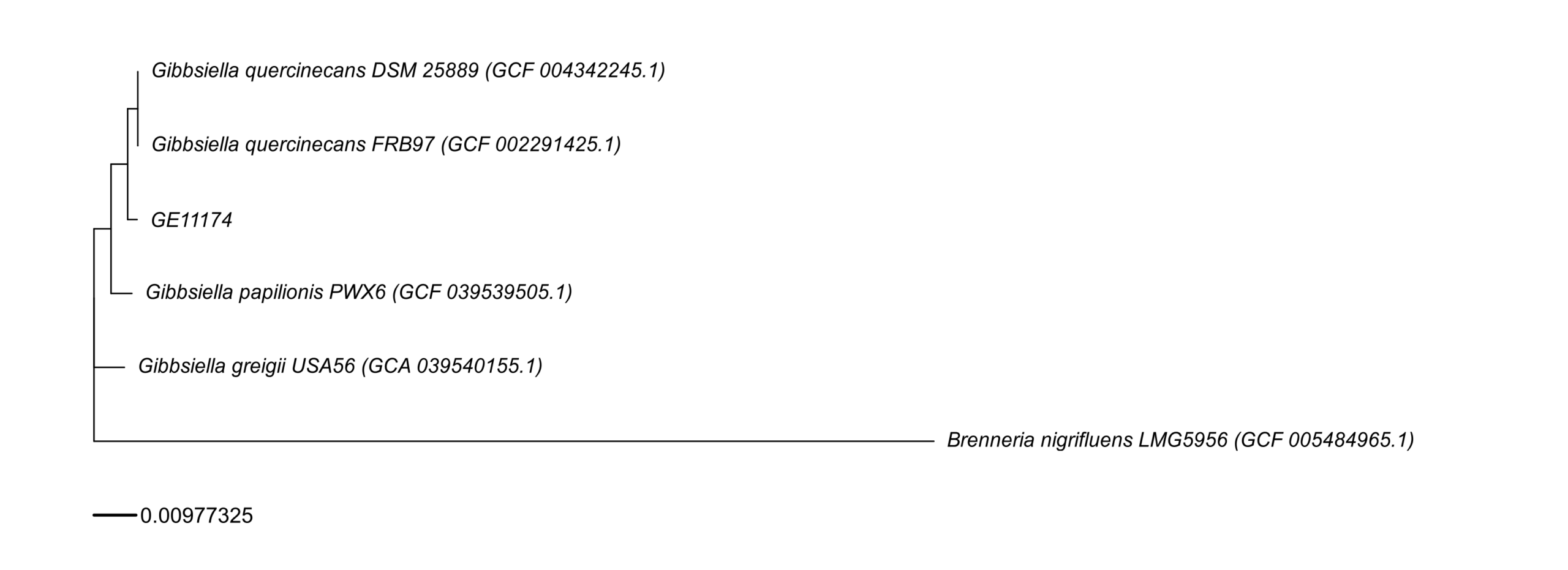
10) fastANI explanation (recorded narrative)
From your tree and the fastANI table, GE11174 is clearly inside the Gibbsiella quercinecans clade, and far from the outgroup (Brenneria nigrifluens). The ANI values quantify that same pattern.
1) Outgroup check (sanity)
-
GE11174 vs Brenneria nigrifluens (GCF_005484965.1): ANI 79.12% (597/1890 fragments)
- 79% ANI is way below any species boundary → not the same genus/species.
- On the tree, Brenneria sits on a long branch as the outgroup, consistent with this deep divergence.
- The relatively low matched fragments (597/1890) also fits “distant genomes” (fewer orthologous regions pass the ANI mapping filters).
2) Species-level placement of GE11174
A common rule of thumb you quoted is correct: ANI ≥ 95–96% ⇒ same species.
Compare GE11174 to the Gibbsiella references:
-
vs GCA_039540155.1 (Gibbsiella greigii USA56): 95.96% (1547/1890)
- Right at the boundary. This suggests “close but could be different species” or “taxonomy/labels may not reflect true species boundaries” depending on how those genomes are annotated.
- On the tree, G. greigii is outside the quercinecans group but not hugely far, which matches “borderline ANI”.
-
vs GCF_039539505.1 (Gibbsiella papilionis PWX6): 97.22% (1588/1890)
-
vs GCF_004342245.1 (G. quercinecans DSM 25889): 98.09% (1599/1890)
-
vs GCF_002291425.1 (G. quercinecans FRB97): 98.13% (1622/1890)
These are all comfortably above 96%, especially the two quercinecans genomes (~98.1%). That strongly supports:
GE11174 belongs to the same species as Gibbsiella quercinecans (and is closer to quercinecans references than to greigii).
3) Closest reference and “same strain?” question
GE11174’s closest by ANI in your list is:
- FRB97 (GCF_002291425.1): 98.1285%
- DSM 25889 (GCF_004342245.1): 98.0889%
- Next: PWX6 97.2172%
These differences are small, but 98.1% ANI is not “same strain” evidence by itself. Within a species, different strains commonly sit anywhere from ~96–99.9% ANI depending on diversity. To claim “same strain / very recent transmission,” people usually look for much tighter genome-wide similarity:
- core-genome SNP distance (often single digits to tens, depending on organism and context)
- cgMLST allele differences
- recombination filtering (if relevant)
- assembly QC/contamination checks
- and confirming that alignment/ANI coverage is high and not biased by missing regions
Your fragment matches (e.g., 1622/1890 for FRB97) are reasonably high, supporting that the ANI is meaningful, but it still doesn’t equate to “same strain.”
4) How to phrase the combined interpretation (tree + ANI)
A clear summary you can use:
- The phylogenetic tree places GE11174 within the Gibbsiella quercinecans lineage, with Brenneria nigrifluens as a distant outgroup.
-
fastANI supports this:
- ~98.1% ANI to G. quercinecans FRB97 and DSM 25889 → strong same-species support.
- 97.2% to G. papilionis → still same-species range, but more distant than the quercinecans references.
- 95.96% to G. greigii → borderline; consistent with being a close neighboring lineage but not the best species match for GE11174.
- 79.1% to Brenneria → confirms it is an appropriate outgroup and far outside the species/genus boundary.
- Therefore, GE11174 is very likely Gibbsiella quercinecans (species-level), and appears most similar to FRB97/DSM 25889, but additional high-resolution analyses are required to assess “same strain.”
If you want, paste the fastANI line for GE11174 vs GE11174? (or run fastANI against a broader set), and/or your core SNP distances from the Roary alignment, and I can help you write a tighter “strain-level” conclusion.
11) Compare to the next closest isolate (pairwise alignment) — nf-core/pairgenomealign
conda deactivate

nextflow run nf-core/pairgenomealign -r 2.2.2 -profile docker \
  --target GE11174.fasta \
  --input samplesheet.csv \
  --outdir pairgenomealign_out \
  --igenomes_base /mnt/nvme1n1p1/igenomes \
  --genome GRCh38
Recorded TODO:
#TODO_NEXT_MONDAY: * phylogenetic tree + fastaANI + nf-core/pairgenomealign (compare to the closest isoalte https://nf-co.re/pairgenomealign/2.2.1/)
- summarize all results with a mail to send them back, mentioned that we can submit the genome to NCBI to obtain a high-quality annotation. What strain name would you like to assign to this isolate?
- If they agree, I can submit the two new isolates to the NCBI-database!
12) Submit both sequences in a batch to NCBI-server! (planned step)
Recorded as:
- submit both sequences in a batch to NCBI-server!
13) Find the closest isolate from GenBank (robust approach) for STEP_7
13.1 Download all available Gibbsiella genomes
# download all available genomes for the genus Gibbsiella (includes assemblies + metadata)
# --assembly-level: must be 'chromosome', 'complete', 'contig', 'scaffold'
datasets download genome taxon Gibbsiella --include genome,gff3,gbff --assembly-level complete,chromosome,scaffold --filename gibbsiella.zip
unzip -q gibbsiella.zip -d gibbsiella_ncbi

mamba activate /home/jhuang/miniconda3/envs/bengal3_ac3
13.2 Mash sketching + nearest neighbors
# make a Mash sketch of your isolate
mash sketch -o isolate bacass_out/Unicycler/GE11174.scaffolds.fa

# sketch all reference genomes (example path—adjust)
find gibbsiella_ncbi -name "*.fna" -o -name "*.fasta" > refs.txt
mash sketch -o refs -l refs.txt

# get closest genomes
mash dist isolate.msh refs.msh | sort -gk3 | head -n 20 > top20_mash.txt
Recorded interpretation:
-
Best hits to
GE11174.scaffolds.faare:- GCA/GCF_002291425.1 (GenBank + RefSeq copies of the same assembly)
- GCA/GCF_004342245.1 (same duplication pattern)
- GCA/GCF_047901425.1 (FRB97; also duplicated)
- Mash distances ~0.018–0.020 are very close (typically same species; often within-species).
p-values are underflow formatting (extremely significant).
13.3 Remove duplicates (GCA vs GCF)
Goal: keep one of each duplicated assembly (prefer GCF if available).
Example snippet recorded:
# Take your top hits, prefer GCF over GCA
cat top20_mash.txt \
  | awk '{print $2}' \
  | sed 's|/GCA_.*||; s|/GCF_.*||' \
  | sort -u
Manual suggestion recorded:
- keep
GCF_002291425.1(dropGCA_002291425.1) - keep
GCF_004342245.1 - keep
GCF_047901425.1 - optionally keep
GCA_032062225.1if it’s truly different and you want a more distant ingroup point
Appendix — Complete attached code (standalone)
Below are the full contents of the attached scripts exactly as provided, so this post can be used standalone in the future.
Note: You mentioned “keep all information of input” and “attach all complete code at the end.” I’ve included all scripts that are currently attached in this chat. If there are additional scripts you meant to attach (e.g.,
run_resistome_virulome*.sh,regenerate_labels.sh,export_table1_stats_to_excel_py36_compat.py, etc.), please upload them and I’ll append them here too.
File: build_wgs_tree_fig3B.sh
#!/usr/bin/env bash
set -euo pipefail

# build_wgs_tree_fig3B.sh
#
# Purpose:
#   Build a core-genome phylogenetic tree and a publication-style plot similar to Fig 3B.
#
# Usage:
#   ./build_wgs_tree_fig3B.sh            # full run
#   ./build_wgs_tree_fig3B.sh plot-only  # only regenerate the plot from existing outputs
#
# Requirements:
#   - Conda env with required tools. Set ENV_NAME to conda env path.
#   - NCBI datasets and/or Entrez usage requires NCBI_EMAIL.
#   - Roary, Prokka, RAxML-NG, MAFFT, R packages for plotting.
#
# Environment variables:
#   ENV_NAME      : path to conda env (e.g., /home/jhuang/miniconda3/envs/bengal3_ac3)
#   NCBI_EMAIL    : email for Entrez calls
#   THREADS       : default threads
#
# Inputs:
#   - targets.tsv: list of target accessions (if used in resolve step)
#   - local isolate genome fasta
#
# Outputs:
#   work_wgs_tree/...
#
# NOTE:
#   If plotting packages are missing in ENV_NAME, run plot-only under an R-capable env (e.g., r_env).

SCRIPT_DIR="$(cd "$(dirname "${BASH_SOURCE[0]}")" && pwd)"
MODE="${1:-full}"

THREADS="${THREADS:-8}"
WORKDIR="${WORKDIR:-work_wgs_tree}"

# Activate conda env if provided
if [[ -n "${ENV_NAME:-}" ]]; then
  # shellcheck disable=SC1090
  source "$(conda info --base)/etc/profile.d/conda.sh"
  conda activate "${ENV_NAME}"
fi

mkdir -p "${WORKDIR}"
mkdir -p "${WORKDIR}/logs"

log() {
  echo "[$(date '+%F %T')] $*" >&2
}

# ------------------------------------------------------------------------------
# Helper: check command exists
need_cmd() {
  command -v "$1" >/dev/null 2>&1 || {
    echo "ERROR: required command '$1' not found in PATH" >&2
    exit 1
  }
}

# ------------------------------------------------------------------------------
# Tool checks (plot-only skips some)
if [[ "${MODE}" != "plot-only" ]]; then
  need_cmd python
  need_cmd roary
  need_cmd raxml-ng
  need_cmd prokka
  need_cmd mafft
  need_cmd awk
  need_cmd sed
  need_cmd grep
fi

need_cmd Rscript

# ------------------------------------------------------------------------------
# Paths
META_DIR="${WORKDIR}/meta"
GENOMES_DIR="${WORKDIR}/genomes_ncbi"
FASTAS_DIR="${WORKDIR}/fastas"
GFFS_DIR="${WORKDIR}/gffs"
PROKKA_DIR="${WORKDIR}/prokka"
ROARY_DIR="${WORKDIR}/roary"
RAXML_DIR="${WORKDIR}/raxmlng"
PLOT_DIR="${WORKDIR}/plot"

mkdir -p "${META_DIR}" "${GENOMES_DIR}" "${FASTAS_DIR}" "${GFFS_DIR}" "${PROKKA_DIR}" "${ROARY_DIR}" "${RAXML_DIR}" "${PLOT_DIR}"

ACCESSIONS_TSV="${META_DIR}/accessions.tsv"
LABELS_TSV="${PLOT_DIR}/labels.tsv"
CORE_ALIGN_PATH_FILE="${META_DIR}/core_alignment_path.txt"

# ------------------------------------------------------------------------------
# Step: plot only
if [[ "${MODE}" == "plot-only" ]]; then
  log "Running in plot-only mode..."

  # If labels file isn't present, try generating a minimal one
  if [[ ! -s "${LABELS_TSV}" ]]; then
    log "labels.tsv not found. Creating a placeholder labels.tsv (edit as needed)."
    {
      echo -e "accession\tdisplay"
      if [[ -d "${FASTAS_DIR}" ]]; then
        for f in "${FASTAS_DIR}"/*.fna "${FASTAS_DIR}"/*.fa "${FASTAS_DIR}"/*.fasta 2>/dev/null; do
          [[ -e "$f" ]] || continue
          bn="$(basename "$f")"
          acc="${bn%%.*}"
          echo -e "${acc}\t${acc}"
        done
      fi
    } > "${LABELS_TSV}"
  fi

  # Plot using plot_tree_v4.R if present; otherwise fall back to plot_tree.R
  PLOT_SCRIPT="${PLOT_DIR}/plot_tree_v4.R"
  if [[ ! -f "${PLOT_SCRIPT}" ]]; then
    PLOT_SCRIPT="${SCRIPT_DIR}/plot_tree_v4.R"
  fi

  if [[ ! -f "${PLOT_SCRIPT}" ]]; then
    echo "ERROR: plot_tree_v4.R not found" >&2
    exit 1
  fi

  SUPPORT_FILE="${RAXML_DIR}/core.raxml.support"
  if [[ ! -f "${SUPPORT_FILE}" ]]; then
    echo "ERROR: Support file not found: ${SUPPORT_FILE}" >&2
    exit 1
  fi

  OUTPDF="${PLOT_DIR}/core_tree.pdf"
  OUTPNG="${PLOT_DIR}/core_tree.png"
  ROOT_N=6

  log "Plotting tree..."
  Rscript "${PLOT_SCRIPT}" \
    "${SUPPORT_FILE}" \
    "${LABELS_TSV}" \
    "${ROOT_N}" \
    "${OUTPDF}" \
    "${OUTPNG}"

  log "Done (plot-only). Outputs: ${OUTPDF} ${OUTPNG}"
  exit 0
fi

# ------------------------------------------------------------------------------
# Full pipeline
log "Running full pipeline..."

# ------------------------------------------------------------------------------
# Config / expected inputs
TARGETS_TSV="${SCRIPT_DIR}/targets.tsv"
RESOLVED_TSV="${SCRIPT_DIR}/resolved_accessions.tsv"
ISOLATE_FASTA="${SCRIPT_DIR}/GE11174.fasta"

# If caller has different locations, let them override
TARGETS_TSV="${TARGETS_TSV_OVERRIDE:-${TARGETS_TSV}}"
RESOLVED_TSV="${RESOLVED_TSV_OVERRIDE:-${RESOLVED_TSV}}"
ISOLATE_FASTA="${ISOLATE_FASTA_OVERRIDE:-${ISOLATE_FASTA}}"

# ------------------------------------------------------------------------------
# Step 1: Resolve best assemblies (if targets.tsv exists)
if [[ -f "${TARGETS_TSV}" ]]; then
  log "Resolving best assemblies from targets.tsv..."
  if [[ -z "${NCBI_EMAIL:-}" ]]; then
    echo "ERROR: NCBI_EMAIL is required for Entrez calls" >&2
    exit 1
  fi
  python "${SCRIPT_DIR}/resolve_best_assemblies_entrez.py" "${TARGETS_TSV}" "${RESOLVED_TSV}"
else
  log "targets.tsv not found; assuming resolved_accessions.tsv already exists"
fi

if [[ ! -s "${RESOLVED_TSV}" ]]; then
  echo "ERROR: resolved_accessions.tsv not found or empty: ${RESOLVED_TSV}" >&2
  exit 1
fi

# ------------------------------------------------------------------------------
# Step 2: Prepare accessions.tsv for downstream steps
log "Preparing accessions.tsv..."
{
  echo -e "label\taccession"
  awk -F'\t' 'NR>1 {print $1"\t"$2}' "${RESOLVED_TSV}"
} > "${ACCESSIONS_TSV}"

# ------------------------------------------------------------------------------
# Step 3: Download genomes (NCBI datasets if available)
log "Downloading genomes (if needed)..."
need_cmd datasets
need_cmd unzip

while IFS=$'\t' read -r label acc; do
  [[ "${label}" == "label" ]] && continue
  [[ -z "${acc}" ]] && continue

  OUTZIP="${GENOMES_DIR}/${acc}.zip"
  OUTDIR="${GENOMES_DIR}/${acc}"

  if [[ -d "${OUTDIR}" ]]; then
    log "  ${acc}: already downloaded"
    continue
  fi

  log "  ${acc}: downloading..."
  datasets download genome accession "${acc}" --include genome --filename "${OUTZIP}" \
    > "${WORKDIR}/logs/datasets_${acc}.stdout.txt" \
    2> "${WORKDIR}/logs/datasets_${acc}.stderr.txt" || {
      echo "ERROR: datasets download failed for ${acc}. See logs." >&2
      exit 1
    }

  mkdir -p "${OUTDIR}"
  unzip -q "${OUTZIP}" -d "${OUTDIR}"
done < "${ACCESSIONS_TSV}"

# ------------------------------------------------------------------------------
# Step 4: Collect FASTA files
log "Collecting FASTA files..."
rm -f "${FASTAS_DIR}"/* 2>/dev/null || true

while IFS=$'\t' read -r label acc; do
  [[ "${label}" == "label" ]] && continue
  OUTDIR="${GENOMES_DIR}/${acc}"
  fna="$(find "${OUTDIR}" -name "*.fna" | head -n 1 || true)"
  if [[ -z "${fna}" ]]; then
    echo "ERROR: no .fna found for ${acc} in ${OUTDIR}" >&2
    exit 1
  fi
  cp -f "${fna}" "${FASTAS_DIR}/${acc}.fna"
done < "${ACCESSIONS_TSV}"

# Add isolate
if [[ -f "${ISOLATE_FASTA}" ]]; then
  cp -f "${ISOLATE_FASTA}" "${FASTAS_DIR}/GE11174.fna"
else
  log "WARNING: isolate fasta not found at ${ISOLATE_FASTA}; skipping"
fi

# ------------------------------------------------------------------------------
# Step 5: Run Prokka on each genome
log "Running Prokka..."
for f in "${FASTAS_DIR}"/*.fna; do
  bn="$(basename "${f}")"
  acc="${bn%.fna}"
  out="${PROKKA_DIR}/${acc}"

  if [[ -d "${out}" && -s "${out}/${acc}.gff" ]]; then
    log "  ${acc}: prokka output exists"
    continue
  fi

  mkdir -p "${out}"
  log "  ${acc}: prokka..."
  prokka --outdir "${out}" --prefix "${acc}" --cpus "${THREADS}" "${f}" \
    > "${WORKDIR}/logs/prokka_${acc}.stdout.txt" \
    2> "${WORKDIR}/logs/prokka_${acc}.stderr.txt"
done

# ------------------------------------------------------------------------------
# Step 6: Collect GFFs for Roary
log "Collecting GFFs..."
rm -f "${GFFS_DIR}"/*.gff 2>/dev/null || true
for d in "${PROKKA_DIR}"/*; do
  [[ -d "${d}" ]] || continue
  acc="$(basename "${d}")"
  gff="${d}/${acc}.gff"
  if [[ -f "${gff}" ]]; then
    cp -f "${gff}" "${GFFS_DIR}/${acc}.gff"
  else
    log "WARNING: missing GFF for ${acc}"
  fi
done

# ------------------------------------------------------------------------------
# Step 7: Roary
log "Running Roary..."
ROARY_OUT="${WORKDIR}/roary_$(date +%s)"
mkdir -p "${ROARY_OUT}"
roary -e --mafft -p "${THREADS}" -cd 95 -i 95 \
  -f "${ROARY_OUT}" \
  "${GFFS_DIR}"/*.gff \
  > "${WORKDIR}/logs/roary.stdout.txt" \
  2> "${WORKDIR}/logs/roary.stderr.txt"

CORE_ALN="${ROARY_OUT}/core_gene_alignment.aln"
if [[ ! -f "${CORE_ALN}" ]]; then
  echo "ERROR: core alignment not found: ${CORE_ALN}" >&2
  exit 1
fi
readlink -f "${CORE_ALN}" > "${CORE_ALIGN_PATH_FILE}"

# ------------------------------------------------------------------------------
# Step 8: RAxML-NG
log "Running RAxML-NG..."
rm -rf "${RAXML_DIR}"
mkdir -p "${RAXML_DIR}"
raxml-ng --all \
  --msa "$(cat "${CORE_ALIGN_PATH_FILE}")" \
  --model GTR+G \
  --bs-trees 1000 \
  --threads "${THREADS}" \
  --prefix "${RAXML_DIR}/core" \
  > "${WORKDIR}/logs/raxml.stdout.txt" \
  2> "${WORKDIR}/logs/raxml.stderr.txt"

SUPPORT_FILE="${RAXML_DIR}/core.raxml.support"
if [[ ! -f "${SUPPORT_FILE}" ]]; then
  echo "ERROR: RAxML support file not found: ${SUPPORT_FILE}" >&2
  exit 1
fi

# ------------------------------------------------------------------------------
# Step 9: Generate labels.tsv (basic)
log "Generating labels.tsv..."
{
  echo -e "accession\tdisplay"
  echo -e "GE11174\tGE11174"
  while IFS=$'\t' read -r label acc; do
    [[ "${label}" == "label" ]] && continue
    echo -e "${acc}\t${label} (${acc})"
  done < "${ACCESSIONS_TSV}"
} > "${LABELS_TSV}"

log "NOTE: You may want to manually edit ${LABELS_TSV} for publication display names."

# ------------------------------------------------------------------------------
# Step 10: Plot
log "Plotting..."
PLOT_SCRIPT="${SCRIPT_DIR}/plot_tree_v4.R"
OUTPDF="${PLOT_DIR}/core_tree.pdf"
OUTPNG="${PLOT_DIR}/core_tree.png"
ROOT_N=6

Rscript "${PLOT_SCRIPT}" \
  "${SUPPORT_FILE}" \
  "${LABELS_TSV}" \
  "${ROOT_N}" \
  "${OUTPDF}" \
  "${OUTPNG}" \
  > "${WORKDIR}/logs/plot.stdout.txt" \
  2> "${WORKDIR}/logs/plot.stderr.txt"

log "Done. Outputs:"
log "  Tree support: ${SUPPORT_FILE}"
log "  Labels:       ${LABELS_TSV}"
log "  Plot PDF:     ${OUTPDF}"
log "  Plot PNG:     ${OUTPNG}"
File: resolve_best_assemblies_entrez.py
#!/usr/bin/env python3
# -*- coding: utf-8 -*-

"""
resolve_best_assemblies_entrez.py

Resolve a "best" assembly accession for a list of target taxa / accessions using NCBI Entrez.

Usage:
  ./resolve_best_assemblies_entrez.py targets.tsv resolved_accessions.tsv

Input (targets.tsv):
  TSV with at least columns:
    label
<tab> query
  Where "query" can be an organism name, taxid, or an assembly/accession hint.

Output (resolved_accessions.tsv):
  TSV with columns:
    label
<tab> accession <tab> organism <tab> assembly_name <tab> assembly_level <tab> refseq_category

Requires:
  - BioPython (Entrez)
  - NCBI_EMAIL environment variable (or set in script)
"""

import os
import sys
import time
import csv
from typing import Dict, List, Optional, Tuple

try:
    from Bio import Entrez
except ImportError:
    sys.stderr.write("ERROR: Biopython is required (Bio.Entrez)\n")
    sys.exit(1)

def eprint(*args, **kwargs):
    print(*args, file=sys.stderr, **kwargs)

def read_targets(path: str) -> List[Tuple[str, str]]:
    rows: List[Tuple[str, str]] = []
    with open(path, "r", newline="") as fh:
        reader = csv.reader(fh, delimiter="\t")
        for i, r in enumerate(reader, start=1):
            if not r:
                continue
            if i == 1 and r[0].lower() in ("label", "name"):
                # header
                continue
            if len(r) < 2:
                continue
            label = r[0].strip()
            query = r[1].strip()
            if label and query:
                rows.append((label, query))
    return rows

def entrez_search(db: str, term: str, retmax: int = 20) -> List[str]:
    handle = Entrez.esearch(db=db, term=term, retmax=retmax)
    res = Entrez.read(handle)
    handle.close()
    return res.get("IdList", [])

def entrez_summary(db: str, ids: List[str]):
    if not ids:
        return []
    handle = Entrez.esummary(db=db, id=",".join(ids), retmode="xml")
    res = Entrez.read(handle)
    handle.close()
    return res

def pick_best_assembly(summaries) -> Optional[Dict]:
    """
    Heuristics:
      Prefer RefSeq (refseq_category != 'na'), prefer higher assembly level:
        complete genome > chromosome > scaffold > contig
      Then prefer latest / highest quality where possible.
    """
    if not summaries:
        return None

    level_rank = {
        "Complete Genome": 4,
        "Chromosome": 3,
        "Scaffold": 2,
        "Contig": 1
    }

    def score(s: Dict) -> Tuple[int, int, int]:
        refcat = s.get("RefSeq_category", "na")
        is_refseq = 1 if (refcat and refcat.lower() != "na") else 0
        level = s.get("AssemblyStatus", "")
        lvl = level_rank.get(level, 0)
        # Prefer latest submit date (YYYY/MM/DD)
        submit = s.get("SubmissionDate", "0000/00/00")
        try:
            y, m, d = submit.split("/")
            date_int = int(y) * 10000 + int(m) * 100 + int(d)
        except Exception:
            date_int = 0
        return (is_refseq, lvl, date_int)

    best = max(summaries, key=score)
    return best

def resolve_query(label: str, query: str) -> Optional[Dict]:
    # If query looks like an assembly accession, search directly.
    term = query
    if query.startswith("GCA_") or query.startswith("GCF_"):
        term = f"{query}[Assembly Accession]"

    ids = entrez_search(db="assembly", term=term, retmax=50)
    if not ids:
        # Try organism name search
        term2 = f"{query}[Organism]"
        ids = entrez_search(db="assembly", term=term2, retmax=50)

    if not ids:
        eprint(f"WARNING: no assembly hits for {label} / {query}")
        return None

    summaries = entrez_summary(db="assembly", ids=ids)
    best = pick_best_assembly(summaries)
    if not best:
        eprint(f"WARNING: could not pick best assembly for {label} / {query}")
        return None

    # Extract useful fields
    acc = best.get("AssemblyAccession", "")
    org = best.get("Organism", "")
    name = best.get("AssemblyName", "")
    level = best.get("AssemblyStatus", "")
    refcat = best.get("RefSeq_category", "")

    return {
        "label": label,
        "accession": acc,
        "organism": org,
        "assembly_name": name,
        "assembly_level": level,
        "refseq_category": refcat
    }

def main():
    if len(sys.argv) != 3:
        eprint("Usage: resolve_best_assemblies_entrez.py targets.tsv resolved_accessions.tsv")
        sys.exit(1)

    targets_path = sys.argv[1]
    out_path = sys.argv[2]

    email = os.environ.get("NCBI_EMAIL") or os.environ.get("ENTREZ_EMAIL")
    if not email:
        eprint("ERROR: please set NCBI_EMAIL environment variable (e.g., export NCBI_EMAIL='you@domain')")
        sys.exit(1)
    Entrez.email = email

    targets = read_targets(targets_path)
    if not targets:
        eprint("ERROR: no targets found in input TSV")
        sys.exit(1)

    out_rows: List[Dict] = []
    for label, query in targets:
        eprint(f"Resolving: {label}\t{query}")
        res = resolve_query(label, query)
        if res:
            out_rows.append(res)
        time.sleep(0.34)  # be nice to NCBI

    with open(out_path, "w", newline="") as fh:
        w = csv.writer(fh, delimiter="\t")
        w.writerow(["label", "accession", "organism", "assembly_name", "assembly_level", "refseq_category"])
        for r in out_rows:
            w.writerow([
                r.get("label", ""),
                r.get("accession", ""),
                r.get("organism", ""),
                r.get("assembly_name", ""),
                r.get("assembly_level", ""),
                r.get("refseq_category", "")
            ])

    eprint(f"Wrote: {out_path} ({len(out_rows)} rows)")

if __name__ == "__main__":
    main()
File: make_table1_GE11174.sh
#!/usr/bin/env bash
set -euo pipefail

# make_table1_GE11174.sh
#
# Generate a "Table 1" summary for sample GE11174:
# - sequencing summary (reads, mean length, etc.)
# - assembly stats
# - BUSCO, N50, etc.
#
# Expects to be run with:
#   ENV_NAME=gunc_env AUTO_INSTALL=1 THREADS=32 ~/Scripts/make_table1_GE11174.sh
#
# This script writes work products to:
#   table1_GE11174_work/

SAMPLE="${SAMPLE:-GE11174}"
THREADS="${THREADS:-8}"
WORKDIR="${WORKDIR:-table1_${SAMPLE}_work}"

AUTO_INSTALL="${AUTO_INSTALL:-0}"
ENV_NAME="${ENV_NAME:-}"

log() {
  echo "[$(date '+%F %T')] $*" >&2
}

# Activate conda env if requested
if [[ -n "${ENV_NAME}" ]]; then
  # shellcheck disable=SC1090
  source "$(conda info --base)/etc/profile.d/conda.sh"
  conda activate "${ENV_NAME}"
fi

mkdir -p "${WORKDIR}"
mkdir -p "${WORKDIR}/logs"

# ------------------------------------------------------------------------------
# Basic tool checks
need_cmd() {
  command -v "$1" >/dev/null 2>&1 || {
    echo "ERROR: required command '$1' not found in PATH" >&2
    exit 1
  }
}

need_cmd awk
need_cmd grep
need_cmd sed
need_cmd wc
need_cmd python

# Optional tools
if command -v seqkit >/dev/null 2>&1; then
  HAVE_SEQKIT=1
else
  HAVE_SEQKIT=0
fi

if command -v pigz >/dev/null 2>&1; then
  HAVE_PIGZ=1
else
  HAVE_PIGZ=0
fi

# ------------------------------------------------------------------------------
# Inputs
RAWREADS="${RAWREADS:-${SAMPLE}.rawreads.fastq.gz}"
ASM_FASTA="${ASM_FASTA:-${SAMPLE}.fasta}"

if [[ ! -f "${RAWREADS}" ]]; then
  log "WARNING: raw reads file not found: ${RAWREADS}"
fi

if [[ ! -f "${ASM_FASTA}" ]]; then
  log "WARNING: assembly fasta not found: ${ASM_FASTA}"
fi

# ------------------------------------------------------------------------------
# Sequencing summary
log "Computing sequencing summary..."
READS_N="NA"
MEAN_LEN="NA"

if [[ -f "${RAWREADS}" ]]; then
  if [[ "${HAVE_PIGZ}" -eq 1 ]]; then
    READS_N="$(pigz -dc "${RAWREADS}" | awk 'END{print NR/4}')"
  else
    READS_N="$(gzip -dc "${RAWREADS}" | awk 'END{print NR/4}')"
  fi

  if [[ "${HAVE_SEQKIT}" -eq 1 ]]; then
    # parse seqkit stats output
    MEAN_LEN="$(seqkit stats "${RAWREADS}" | awk 'NR==2{print $8}')"
  fi
fi

# ------------------------------------------------------------------------------
# Assembly stats (simple)
log "Computing assembly stats..."
ASM_SIZE="NA"
ASM_CONTIGS="NA"

if [[ -f "${ASM_FASTA}" ]]; then
  # Count contigs and sum length
  ASM_CONTIGS="$(grep -c '^>' "${ASM_FASTA}" || true)"
  ASM_SIZE="$(grep -v '^>' "${ASM_FASTA}" | tr -d '\n' | wc -c | awk '{print $1}')"
fi

# ------------------------------------------------------------------------------
# Output a basic TSV summary (can be expanded)
OUT_TSV="${WORKDIR}/table1_${SAMPLE}.tsv"
{
  echo -e "sample\treads_total\tmean_read_length_bp\tassembly_contigs\tassembly_size_bp"
  echo -e "${SAMPLE}\t${READS_N}\t${MEAN_LEN}\t${ASM_CONTIGS}\t${ASM_SIZE}"
} > "${OUT_TSV}"

log "Wrote: ${OUT_TSV}"
File: export_table1_stats_to_excel_py36_compat.py
#!/usr/bin/env python3
# -*- coding: utf-8 -*-
"""
Export a comprehensive Excel workbook from a Table1 pipeline workdir.
Python 3.6 compatible (no PEP604 unions, no builtin generics).
Requires: openpyxl

Sheets (as available):
- Summary
- Table1 (if Table1_*.tsv exists)
- QUAST_report (report.tsv)
- QUAST_metrics (metric/value)
- Mosdepth_summary (*.mosdepth.summary.txt)
- CheckM (checkm_summary.tsv)
- GUNC_* (all .tsv under gunc/out)
- File_Inventory (relative path, size, mtime; optional md5 for small files)
- Run_log_preview (head/tail of latest log under workdir/logs or workdir/*/logs)
"""

from __future__ import print_function

import argparse
import csv
import hashlib
import os
import sys
import time
from pathlib import Path

try:
    from openpyxl import Workbook
    from openpyxl.utils import get_column_letter
except ImportError:
    sys.stderr.write("ERROR: openpyxl is required. Install with:\n"
                     "  conda install -c conda-forge openpyxl\n")
    raise

MAX_XLSX_ROWS = 1048576

def safe_sheet_name(name, used):
    # Excel: <=31 chars, cannot contain: : \ / ? * [ ]
    bad = r'[:\\/?*\[\]]'
    base = name.strip() or "Sheet"
    base = __import__("re").sub(bad, "_", base)
    base = base[:31]
    if base not in used:
        used.add(base)
        return base
    # make unique with suffix
    for i in range(2, 1000):
        suffix = "_%d" % i
        cut = 31 - len(suffix)
        candidate = (base[:cut] + suffix)
        if candidate not in used:
            used.add(candidate)
            return candidate
    raise RuntimeError("Too many duplicate sheet names for base=%s" % base)

def autosize(ws, max_width=60):
    for col in ws.columns:
        max_len = 0
        col_letter = get_column_letter(col[0].column)
        for cell in col:
            v = cell.value
            if v is None:
                continue
            s = str(v)
            if len(s) > max_len:
                max_len = len(s)
        ws.column_dimensions[col_letter].width = min(max_width, max(10, max_len + 2))

def write_table(ws, header, rows, max_rows=None):
    if header:
        ws.append(header)
    count = 0
    for r in rows:
        ws.append(r)
        count += 1
        if max_rows is not None and count >= max_rows:
            break

def read_tsv(path, max_rows=None):
    header = []
    rows = []
    with path.open("r", newline="") as f:
        reader = csv.reader(f, delimiter="\t")
        for i, r in enumerate(reader):
            if i == 0:
                header = r
                continue
            rows.append(r)
            if max_rows is not None and len(rows) >= max_rows:
                break
    return header, rows

def read_text_table(path, max_rows=None):
    # for mosdepth summary (tsv with header)
    return read_tsv(path, max_rows=max_rows)

def md5_file(path, chunk=1024*1024):
    h = hashlib.md5()
    with path.open("rb") as f:
        while True:
            b = f.read(chunk)
            if not b:
                break
            h.update(b)
    return h.hexdigest()

def find_latest_log(workdir):
    candidates = []
    # common locations
    for p in [workdir / "logs", workdir / "log", workdir / "Logs"]:
        if p.exists():
            candidates.extend(p.glob("*.log"))
    # nested logs
    candidates.extend(workdir.glob("**/logs/*.log"))
    if not candidates:
        return None
    candidates.sort(key=lambda x: x.stat().st_mtime, reverse=True)
    return candidates[0]

def add_summary_sheet(wb, used, info_items):
    ws = wb.create_sheet(title=safe_sheet_name("Summary", used))
    ws.append(["Key", "Value"])
    for k, v in info_items:
        ws.append([k, v])
    autosize(ws)

def add_log_preview(wb, used, log_path, head_n=80, tail_n=120):
    if log_path is None or not log_path.exists():
        return
    ws = wb.create_sheet(title=safe_sheet_name("Run_log_preview", used))
    ws.append(["Log path", str(log_path)])
    ws.append([])
    lines = log_path.read_text(errors="replace").splitlines()
    ws.append(["--- HEAD (%d) ---" % head_n])
    for line in lines[:head_n]:
        ws.append([line])
    ws.append([])
    ws.append(["--- TAIL (%d) ---" % tail_n])
    for line in lines[-tail_n:]:
        ws.append([line])
    ws.column_dimensions["A"].width = 120

def add_file_inventory(wb, used, workdir, do_md5=True, md5_max_bytes=200*1024*1024, max_rows=None):
    ws = wb.create_sheet(title=safe_sheet_name("File_Inventory", used))
    ws.append(["relative_path", "size_bytes", "mtime_iso", "md5(optional)"])
    count = 0
    for p in sorted(workdir.rglob("*")):
        if p.is_dir():
            continue
        rel = str(p.relative_to(workdir))
        st = p.stat()
        mtime = time.strftime("%Y-%m-%d %H:%M:%S", time.localtime(st.st_mtime))
        md5 = ""
        if do_md5 and st.st_size <= md5_max_bytes:
            try:
                md5 = md5_file(p)
            except Exception:
                md5 = "ERROR"
        ws.append([rel, st.st_size, mtime, md5])
        count += 1
        if max_rows is not None and count >= max_rows:
            break
    autosize(ws, max_width=80)

def add_tsv_sheet(wb, used, name, path, max_rows=None):
    header, rows = read_tsv(path, max_rows=max_rows)
    ws = wb.create_sheet(title=safe_sheet_name(name, used))
    write_table(ws, header, rows, max_rows=max_rows)
    autosize(ws, max_width=80)

def add_quast_metrics_sheet(wb, used, quast_report_tsv):
    header, rows = read_tsv(quast_report_tsv, max_rows=None)
    if not header or len(header) < 2:
        return
    asm_name = header[1]
    ws = wb.create_sheet(title=safe_sheet_name("QUAST_metrics", used))
    ws.append(["Metric", asm_name])
    for r in rows:
        if not r:
            continue
        metric = r[0]
        val = r[1] if len(r) > 1 else ""
        ws.append([metric, val])
    autosize(ws, max_width=80)

def main():
    ap = argparse.ArgumentParser()
    ap.add_argument("--workdir", required=True, help="workdir produced by pipeline (e.g., table1_GE11174_work)")
    ap.add_argument("--out", required=True, help="output .xlsx")
    ap.add_argument("--sample", default="", help="sample name for summary")
    ap.add_argument("--max-rows", type=int, default=200000, help="max rows per large sheet")
    ap.add_argument("--no-md5", action="store_true", help="skip md5 calculation in File_Inventory")
    args = ap.parse_args()

    workdir = Path(args.workdir).resolve()
    out = Path(args.out).resolve()

    if not workdir.exists():
        sys.stderr.write("ERROR: workdir not found: %s\n" % workdir)
        sys.exit(2)

    wb = Workbook()
    # remove default sheet
    wb.remove(wb.active)
    used = set()

    # Summary info
    info = [
        ("sample", args.sample or ""),
        ("workdir", str(workdir)),
        ("generated_at", time.strftime("%Y-%m-%d %H:%M:%S")),
        ("python", sys.version.replace("\n", " ")),
        ("openpyxl", __import__("openpyxl").__version__),
    ]
    add_summary_sheet(wb, used, info)

    # Table1 TSV (try common names)
    table1_candidates = list(workdir.glob("Table1_*.tsv")) + list(workdir.glob("*.tsv"))
    # Prefer Table1_*.tsv in workdir root
    table1_path = None
    for p in table1_candidates:
        if p.name.startswith("Table1_") and p.suffix == ".tsv":
            table1_path = p
            break
    if table1_path is None:
        # maybe created in cwd, not inside workdir; try alongside workdir
        parent = workdir.parent
        for p in parent.glob("Table1_*.tsv"):
            if args.sample and args.sample in p.name:
                table1_path = p
                break
        if table1_path is None and list(parent.glob("Table1_*.tsv")):
            table1_path = sorted(parent.glob("Table1_*.tsv"))[0]

    if table1_path is not None and table1_path.exists():
        add_tsv_sheet(wb, used, "Table1", table1_path, max_rows=args.max_rows)

    # QUAST
    quast_report = workdir / "quast" / "report.tsv"
    if quast_report.exists():
        add_tsv_sheet(wb, used, "QUAST_report", quast_report, max_rows=args.max_rows)
        add_quast_metrics_sheet(wb, used, quast_report)

    # Mosdepth summary
    for p in sorted((workdir / "map").glob("*.mosdepth.summary.txt")):
        # mosdepth summary is TSV-like
        name = "Mosdepth_" + p.stem.replace(".mosdepth.summary", "")
        add_tsv_sheet(wb, used, name[:31], p, max_rows=args.max_rows)

    # CheckM
    checkm_sum = workdir / "checkm" / "checkm_summary.tsv"
    if checkm_sum.exists():
        add_tsv_sheet(wb, used, "CheckM", checkm_sum, max_rows=args.max_rows)

    # GUNC outputs (all TSV under gunc/out)
    gunc_out = workdir / "gunc" / "out"
    if gunc_out.exists():
        for p in sorted(gunc_out.rglob("*.tsv")):
            rel = str(p.relative_to(gunc_out))
            sheet = "GUNC_" + rel.replace("/", "_").replace("\\", "_").replace(".tsv", "")
            add_tsv_sheet(wb, used, sheet[:31], p, max_rows=args.max_rows)

    # Log preview
    latest_log = find_latest_log(workdir)
    add_log_preview(wb, used, latest_log)

    # File inventory
    add_file_inventory(
        wb, used, workdir,
        do_md5=(not args.no_md5),
        md5_max_bytes=200*1024*1024,
        max_rows=args.max_rows
    )

    # Save
    out.parent.mkdir(parents=True, exist_ok=True)
    wb.save(str(out))
    print("OK: wrote %s" % out)

if __name__ == "__main__":
    main()
File: make_table1_with_excel.sh
#!/usr/bin/env bash
set -euo pipefail

# make_table1_with_excel.sh
#
# Wrapper to run:
#   1) make_table1_* (stats extraction)
#   2) export_table1_stats_to_excel_py36_compat.py
#
# Example:
#   ENV_NAME=gunc_env AUTO_INSTALL=1 THREADS=32 ~/Scripts/make_table1_with_excel.sh

SAMPLE="${SAMPLE:-GE11174}"
THREADS="${THREADS:-8}"
WORKDIR="${WORKDIR:-table1_${SAMPLE}_work}"
OUT_XLSX="${OUT_XLSX:-Comprehensive_${SAMPLE}.xlsx}"

ENV_NAME="${ENV_NAME:-}"
AUTO_INSTALL="${AUTO_INSTALL:-0}"

log() {
  echo "[$(date '+%F %T')] $*" >&2
}

# Activate conda env if requested
if [[ -n "${ENV_NAME}" ]]; then
  # shellcheck disable=SC1090
  source "$(conda info --base)/etc/profile.d/conda.sh"
  conda activate "${ENV_NAME}"
fi

mkdir -p "${WORKDIR}"

# ------------------------------------------------------------------------------
# Locate scripts
SCRIPT_DIR="$(cd "$(dirname "${BASH_SOURCE[0]}")" && pwd)"
MAKE_TABLE1="${MAKE_TABLE1_SCRIPT:-${SCRIPT_DIR}/make_table1_${SAMPLE}.sh}"
EXPORT_PY="${EXPORT_PY_SCRIPT:-${SCRIPT_DIR}/export_table1_stats_to_excel_py36_compat.py}"

# Fallback for naming mismatch (e.g., make_table1_GE11174.sh)
if [[ ! -f "${MAKE_TABLE1}" ]]; then
  MAKE_TABLE1="${SCRIPT_DIR}/make_table1_GE11174.sh"
fi

if [[ ! -f "${MAKE_TABLE1}" ]]; then
  echo "ERROR: make_table1 script not found" >&2
  exit 1
fi

if [[ ! -f "${EXPORT_PY}" ]]; then
  log "WARNING: export_table1_stats_to_excel_py36_compat.py not found next to this script."
  log "         You can set EXPORT_PY_SCRIPT=/path/to/export_table1_stats_to_excel_py36_compat.py"
fi

# ------------------------------------------------------------------------------
# Step 1
log "STEP 1: generating workdir stats..."
ENV_NAME="${ENV_NAME}" AUTO_INSTALL="${AUTO_INSTALL}" THREADS="${THREADS}" SAMPLE="${SAMPLE}" WORKDIR="${WORKDIR}" \
  bash "${MAKE_TABLE1}"

# ------------------------------------------------------------------------------
# Step 2
if [[ -f "${EXPORT_PY}" ]]; then
  log "STEP 2: exporting to Excel..."
  python "${EXPORT_PY}" \
    --workdir "${WORKDIR}" \
    --out "${OUT_XLSX}" \
    --max-rows 200000 \
    --sample "${SAMPLE}"
  log "Wrote: ${OUT_XLSX}"
else
  log "Skipped Excel export (missing export script). Workdir still produced: ${WORKDIR}"
fi
File: merge_amr_sources_by_gene.py
#!/usr/bin/env python3
# -*- coding: utf-8 -*-

"""
merge_amr_sources_by_gene.py

Merge AMR calls from multiple sources (e.g., ABRicate outputs from MEGARes/ResFinder
and RGI/CARD) by gene name, producing a combined table suitable for reporting/export.

This script is intentionally lightweight and focuses on:
- reading tabular ABRicate outputs
- normalizing gene names
- merging into a per-gene summary

Expected inputs/paths are typically set in your working directory structure.
"""

import os
import sys
import csv
from collections import defaultdict
from typing import Dict, List, Tuple

def eprint(*args, **kwargs):
    print(*args, file=sys.stderr, **kwargs)

def read_abricate_tab(path: str) -> List[Dict[str, str]]:
    rows: List[Dict[str, str]] = []
    with open(path, "r", newline="") as fh:
        for line in fh:
            if line.startswith("#") or not line.strip():
                continue
            # ABRicate default is tab-delimited with columns:
            # FILE, SEQUENCE, START, END, STRAND, GENE, COVERAGE, COVERAGE_MAP, GAPS,
            # %COVERAGE, %IDENTITY, DATABASE, ACCESSION, PRODUCT, RESISTANCE
            parts = line.rstrip("\n").split("\t")
            if len(parts) < 12:
                continue
            gene = parts[5].strip()
            rows.append({
                "gene": gene,
                "identity": parts[10].strip(),
                "coverage": parts[9].strip(),
                "db": parts[11].strip(),
                "product": parts[13].strip() if len(parts) > 13 else "",
                "raw": line.rstrip("\n")
            })
    return rows

def normalize_gene(gene: str) -> str:
    g = gene.strip()
    # Add any project-specific normalization rules here
    return g

def merge_sources(sources: List[Tuple[str, str]]) -> Dict[str, Dict[str, List[Dict[str, str]]]]:
    merged: Dict[str, Dict[str, List[Dict[str, str]]]] = defaultdict(lambda: defaultdict(list))
    for src_name, path in sources:
        if not os.path.exists(path):
            eprint(f"WARNING: missing source file: {path}")
            continue
        rows = read_abricate_tab(path)
        for r in rows:
            g = normalize_gene(r["gene"])
            merged[g][src_name].append(r)
    return merged

def write_merged_tsv(out_path: str, merged: Dict[str, Dict[str, List[Dict[str, str]]]]):
    # Flatten into a simple TSV
    with open(out_path, "w", newline="") as fh:
        w = csv.writer(fh, delimiter="\t")
        w.writerow(["gene", "sources", "best_identity", "best_coverage", "notes"])
        for gene, src_map in sorted(merged.items()):
            srcs = sorted(src_map.keys())
            best_id = ""
            best_cov = ""
            notes = []
            # pick best identity/coverage across all hits
            for s in srcs:
                for r in src_map[s]:
                    if not best_id or float(r["identity"]) > float(best_id):
                        best_id = r["identity"]
                    if not best_cov or float(r["coverage"]) > float(best_cov):
                        best_cov = r["coverage"]
                    if r.get("product"):
                        notes.append(f"{s}:{r['product']}")
            w.writerow([gene, ",".join(srcs), best_id, best_cov, "; ".join(notes)])

def main():
    # Default expected layout (customize as needed)
    workdir = os.environ.get("WORKDIR", "resistome_virulence_GE11174")
    sample = os.environ.get("SAMPLE", "GE11174")

    rawdir = os.path.join(workdir, "raw")
    sources = [
        ("MEGARes", os.path.join(rawdir, f"{sample}.megares.tab")),
        ("CARD", os.path.join(rawdir, f"{sample}.card.tab")),
        ("ResFinder", os.path.join(rawdir, f"{sample}.resfinder.tab")),
        ("VFDB", os.path.join(rawdir, f"{sample}.vfdb.tab")),
    ]

    merged = merge_sources(sources)
    out_path = os.path.join(workdir, f"merged_by_gene_{sample}.tsv")
    write_merged_tsv(out_path, merged)
    eprint(f"Wrote merged table: {out_path}")

if __name__ == "__main__":
    main()
File: export_resistome_virulence_to_excel_py36.py
#!/usr/bin/env python3
# -*- coding: utf-8 -*-

"""
export_resistome_virulence_to_excel_py36.py

Export resistome + virulence profiling outputs to an Excel workbook, compatible with
older Python (3.6) style environments.

Typical usage:
  python export_resistome_virulence_to_excel_py36.py \
    --workdir resistome_virulence_GE11174 \
    --sample GE11174 \
    --out Resistome_Virulence_GE11174.xlsx

Requires:
  - openpyxl
"""

import os
import sys
import csv
import argparse
from typing import List, Dict

try:
    from openpyxl import Workbook
except ImportError:
    sys.stderr.write("ERROR: openpyxl is required\n")
    sys.exit(1)

def eprint(*args, **kwargs):
    print(*args, file=sys.stderr, **kwargs)

def read_tab_file(path: str) -> List[List[str]]:
    rows: List[List[str]] = []
    with open(path, "r", newline="") as fh:
        for line in fh:
            if line.startswith("#") or not line.strip():
                continue
            rows.append(line.rstrip("\n").split("\t"))
    return rows

def autosize(ws):
    # basic autosize columns
    for col_cells in ws.columns:
        max_len = 0
        col_letter = col_cells[0].column_letter
        for c in col_cells:
            if c.value is None:
                continue
            max_len = max(max_len, len(str(c.value)))
        ws.column_dimensions[col_letter].width = min(max_len + 2, 60)

def add_sheet_from_tab(wb: Workbook, title: str, path: str):
    ws = wb.create_sheet(title=title)
    if not os.path.exists(path):
        ws.append([f"Missing file: {path}"])
        return
    rows = read_tab_file(path)
    if not rows:
        ws.append(["No rows"])
        return
    for r in rows:
        ws.append(r)
    autosize(ws)

def main():
    ap = argparse.ArgumentParser()
    ap.add_argument("--workdir", required=True)
    ap.add_argument("--sample", required=True)
    ap.add_argument("--out", required=True)
    args = ap.parse_args()

    workdir = args.workdir
    sample = args.sample
    out_xlsx = args.out

    rawdir = os.path.join(workdir, "raw")

    files = {
        "MEGARes": os.path.join(rawdir, f"{sample}.megares.tab"),
        "CARD": os.path.join(rawdir, f"{sample}.card.tab"),
        "ResFinder": os.path.join(rawdir, f"{sample}.resfinder.tab"),
        "VFDB": os.path.join(rawdir, f"{sample}.vfdb.tab"),
        "Merged_by_gene": os.path.join(workdir, f"merged_by_gene_{sample}.tsv"),
    }

    wb = Workbook()
    # Remove default sheet
    default = wb.active
    wb.remove(default)

    for title, path in files.items():
        eprint(f"Adding sheet: {title} <- {path}")
        add_sheet_from_tab(wb, title, path)

    wb.save(out_xlsx)
    eprint(f"Wrote Excel: {out_xlsx}")

if __name__ == "__main__":
    main()
File: plot_tree_v4.R
#!/usr/bin/env Rscript

# plot_tree_v4.R
#
# Plot a RAxML-NG support tree with custom labels.
#
# Args:
#   1) support tree file (e.g., core.raxml.support)
#   2) labels.tsv (columns: accession
<TAB>display)
#   3) root N (numeric, e.g., 6)
#   4) output PDF
#   5) output PNG

suppressPackageStartupMessages({
  library(ape)
  library(ggplot2)
  library(ggtree)
  library(dplyr)
  library(readr)
  library(aplot)
})

args <- commandArgs(trailingOnly=TRUE)
if (length(args) < 5) {
  cat("Usage: plot_tree_v4.R
<support_tree> <labels.tsv> <root_n> <out.pdf> <out.png>\n")
  quit(status=1)
}

support_tree <- args[1]
labels_tsv <- args[2]
root_n <- as.numeric(args[3])
out_pdf <- args[4]
out_png <- args[5]

# Read tree
tr <- read.tree(support_tree)

# Read labels
lab <- read_tsv(labels_tsv, col_types=cols(.default="c"))
colnames(lab) <- c("accession","display")

# Map labels
# Current tip labels may include accession-like tokens.
# We'll try exact match first; otherwise keep original.
tip_map <- setNames(lab$display, lab$accession)
new_labels <- sapply(tr$tip.label, function(x) {
  if (x %in% names(tip_map)) {
    tip_map[[x]]
  } else {
    x
  }
})
tr$tip.label <- new_labels

# Root by nth tip if requested
if (!is.na(root_n) && root_n > 0 && root_n <= length(tr$tip.label)) {
  tr <- root(tr, outgroup=tr$tip.label[root_n], resolve.root=TRUE)
}

# Plot
p <- ggtree(tr) +
  geom_tiplab(size=3) +
  theme_tree2()

# Save
ggsave(out_pdf, plot=p, width=8, height=8)
ggsave(out_png, plot=p, width=8, height=8, dpi=300)

cat(sprintf("Wrote: %s\nWrote: %s\n", out_pdf, out_png))
File: run_resistome_virulome_dedup.sh
#!/usr/bin/env bash
set -Eeuo pipefail

# -------- user inputs --------
ENV_NAME="${ENV_NAME:-bengal3_ac3}"
ASM="${ASM:-GE11174.fasta}"
SAMPLE="${SAMPLE:-GE11174}"
OUTDIR="${OUTDIR:-resistome_virulence_${SAMPLE}}"
THREADS="${THREADS:-16}"

# thresholds (set to 0/0 if you truly want ABRicate defaults)
MINID="${MINID:-90}"
MINCOV="${MINCOV:-60}"
# ----------------------------

log(){ echo "[$(date +'%F %T')] $*" >&2; }
need_cmd(){ command -v "$1" >/dev/null 2>&1; }

activate_env() {
  # shellcheck disable=SC1091
  source "$(conda info --base)/etc/profile.d/conda.sh"
  conda activate "${ENV_NAME}"
}

main(){
  activate_env

  mkdir -p "${OUTDIR}"/{raw,amr,virulence,card,tmp}

  log "Env:    ${ENV_NAME}"
  log "ASM:    ${ASM}"
  log "Sample: ${SAMPLE}"
  log "Outdir: ${OUTDIR}"
  log "ABRicate thresholds: MINID=${MINID} MINCOV=${MINCOV}"

  log "ABRicate DB list:"
  abricate --list | egrep -i "vfdb|resfinder|megares|card" || true

  # Make sure indices exist
  log "Running abricate --setupdb (safe even if already done)..."
  abricate --setupdb

  # ---- ABRicate AMR DBs ----
  log "Running ABRicate: ResFinder"
  abricate --db resfinder --minid "${MINID}" --mincov "${MINCOV}" "${ASM}" > "${OUTDIR}/raw/${SAMPLE}.resfinder.tab"

  log "Running ABRicate: MEGARes"
  abricate --db megares   --minid "${MINID}" --mincov "${MINCOV}" "${ASM}" > "${OUTDIR}/raw/${SAMPLE}.megares.tab"

  # ---- Virulence (VFDB) ----
  log "Running ABRicate: VFDB"
  abricate --db vfdb      --minid "${MINID}" --mincov "${MINCOV}" "${ASM}" > "${OUTDIR}/raw/${SAMPLE}.vfdb.tab"

  # ---- CARD: prefer RGI if available, else ABRicate card ----
  CARD_MODE="ABRicate"
  if need_cmd rgi; then
    log "RGI found. Trying RGI (CARD) ..."
    set +e
    rgi main --input_sequence "${ASM}" --output_file "${OUTDIR}/card/${SAMPLE}.rgi" --input_type contig --num_threads "${THREADS}"
    rc=$?
    set -e
    if [[ $rc -eq 0 ]]; then
      CARD_MODE="RGI"
    else
      log "RGI failed (likely CARD data not installed). Falling back to ABRicate card."
    fi
  fi

  if [[ "${CARD_MODE}" == "ABRicate" ]]; then
    log "Running ABRicate: CARD"
    abricate --db card --minid "${MINID}" --mincov "${MINCOV}" "${ASM}" > "${OUTDIR}/raw/${SAMPLE}.card.tab"
  fi

  # ---- Build deduplicated tables ----
  log "Creating deduplicated AMR/VFDB tables..."

  export OUTDIR SAMPLE CARD_MODE
  python - <<'PY'
import os, re
from pathlib import Path
import pandas as pd
from io import StringIO

outdir = Path(os.environ["OUTDIR"])
sample = os.environ["SAMPLE"]
card_mode = os.environ["CARD_MODE"]

def read_abricate_tab(path: Path, source: str) -> pd.DataFrame:
    if not path.exists() or path.stat().st_size == 0:
        return pd.DataFrame()
    lines=[]
    with path.open("r", errors="replace") as f:
        for line in f:
            if line.startswith("#") or not line.strip():
                continue
            lines.append(line)
    if not lines:
        return pd.DataFrame()
    df = pd.read_csv(StringIO("".join(lines)), sep="\t", dtype=str)
    df.insert(0, "Source", source)
    return df

def to_num(s):
    try:
        return float(str(s).replace("%",""))
    except:
        return None

def normalize_abricate(df: pd.DataFrame, dbname: str) -> pd.DataFrame:
    if df.empty:
        return pd.DataFrame(columns=[
            "Source","Database","Gene","Product","Accession","Contig","Start","End","Strand","Pct_Identity","Pct_Coverage"
        ])
    # Column names vary slightly; handle common ones
    gene = "GENE" if "GENE" in df.columns else None
    prod = "PRODUCT" if "PRODUCT" in df.columns else None
    acc  = "ACCESSION" if "ACCESSION" in df.columns else None
    contig = "SEQUENCE" if "SEQUENCE" in df.columns else ("CONTIG" if "CONTIG" in df.columns else None)
    start = "START" if "START" in df.columns else None
    end   = "END" if "END" in df.columns else None
    strand= "STRAND" if "STRAND" in df.columns else None

    pid = "%IDENTITY" if "%IDENTITY" in df.columns else ("% Identity" if "% Identity" in df.columns else None)
    pcv = "%COVERAGE" if "%COVERAGE" in df.columns else ("% Coverage" if "% Coverage" in df.columns else None)

    out = pd.DataFrame()
    out["Source"] = df["Source"]
    out["Database"] = dbname
    out["Gene"] = df[gene] if gene else ""
    out["Product"] = df[prod] if prod else ""
    out["Accession"] = df[acc] if acc else ""
    out["Contig"] = df[contig] if contig else ""
    out["Start"] = df[start] if start else ""
    out["End"] = df[end] if end else ""
    out["Strand"] = df[strand] if strand else ""
    out["Pct_Identity"] = df[pid] if pid else ""
    out["Pct_Coverage"] = df[pcv] if pcv else ""
    return out

def dedup_best(df: pd.DataFrame, key_cols):
    """Keep best hit per key by highest identity, then coverage, then longest span."""
    if df.empty:
        return df
    # numeric helpers
    df = df.copy()
    df["_pid"] = df["Pct_Identity"].map(to_num)
    df["_pcv"] = df["Pct_Coverage"].map(to_num)

    def span(row):
        try:
            return abs(int(row["End"]) - int(row["Start"])) + 1
        except:
            return 0
    df["_span"] = df.apply(span, axis=1)

    # sort best-first
    df = df.sort_values(by=["_pid","_pcv","_span"], ascending=[False,False,False], na_position="last")
    df = df.drop_duplicates(subset=key_cols, keep="first")
    df = df.drop(columns=["_pid","_pcv","_span"])
    return df

# ---------- AMR inputs ----------
amr_frames = []

# ResFinder (often 0 hits; still okay)
resfinder = outdir / "raw" / f"{sample}.resfinder.tab"
df = read_abricate_tab(resfinder, "ABRicate")
amr_frames.append(normalize_abricate(df, "ResFinder"))

# MEGARes
megares = outdir / "raw" / f"{sample}.megares.tab"
df = read_abricate_tab(megares, "ABRicate")
amr_frames.append(normalize_abricate(df, "MEGARes"))

# CARD: RGI or ABRicate
if card_mode == "RGI":
    # Try common RGI tab outputs
    prefix = outdir / "card" / f"{sample}.rgi"
    rgi_tab = None
    for ext in [".txt",".tab",".tsv"]:
        p = Path(str(prefix) + ext)
        if p.exists() and p.stat().st_size > 0:
            rgi_tab = p
            break
    if rgi_tab is not None:
        rgi = pd.read_csv(rgi_tab, sep="\t", dtype=str)
        out = pd.DataFrame()
        out["Source"] = "RGI"
        out["Database"] = "CARD"
        # Prefer ARO_name/Best_Hit_ARO if present
        out["Gene"] = rgi["ARO_name"] if "ARO_name" in rgi.columns else (rgi["Best_Hit_ARO"] if "Best_Hit_ARO" in rgi.columns else "")
        out["Product"] = rgi["ARO_name"] if "ARO_name" in rgi.columns else ""
        out["Accession"] = rgi["ARO_accession"] if "ARO_accession" in rgi.columns else ""
        out["Contig"] = rgi["Sequence"] if "Sequence" in rgi.columns else ""
        out["Start"] = rgi["Start"] if "Start" in rgi.columns else ""
        out["End"] = rgi["Stop"] if "Stop" in rgi.columns else (rgi["End"] if "End" in rgi.columns else "")
        out["Strand"] = rgi["Orientation"] if "Orientation" in rgi.columns else ""
        out["Pct_Identity"] = rgi["% Identity"] if "% Identity" in rgi.columns else ""
        out["Pct_Coverage"] = rgi["% Coverage"] if "% Coverage" in rgi.columns else ""
        amr_frames.append(out)
else:
    card = outdir / "raw" / f"{sample}.card.tab"
    df = read_abricate_tab(card, "ABRicate")
    amr_frames.append(normalize_abricate(df, "CARD"))

amr_all = pd.concat([x for x in amr_frames if not x.empty], ignore_index=True) if any(not x.empty for x in amr_frames) else pd.DataFrame(
    columns=["Source","Database","Gene","Product","Accession","Contig","Start","End","Strand","Pct_Identity","Pct_Coverage"]
)

# Deduplicate within each (Database,Gene) – this is usually what you want for manuscript tables
amr_dedup = dedup_best(amr_all, key_cols=["Database","Gene"])

# Sort nicely
if not amr_dedup.empty:
    amr_dedup = amr_dedup.sort_values(["Database","Gene"]).reset_index(drop=True)

amr_out = outdir / "Table_AMR_genes_dedup.tsv"
amr_dedup.to_csv(amr_out, sep="\t", index=False)

# ---------- Virulence (VFDB) ----------
vfdb = outdir / "raw" / f"{sample}.vfdb.tab"
vf = read_abricate_tab(vfdb, "ABRicate")
vf_norm = normalize_abricate(vf, "VFDB")

# Dedup within (Gene) for VFDB (or use Database,Gene; Database constant)
vf_dedup = dedup_best(vf_norm, key_cols=["Gene"]) if not vf_norm.empty else vf_norm
if not vf_dedup.empty:
    vf_dedup = vf_dedup.sort_values(["Gene"]).reset_index(drop=True)

vf_out = outdir / "Table_Virulence_VFDB_dedup.tsv"
vf_dedup.to_csv(vf_out, sep="\t", index=False)

print("OK wrote:")
print(" ", amr_out)
print(" ", vf_out)
PY

  log "Done."
  log "Outputs:"
  log "  ${OUTDIR}/Table_AMR_genes_dedup.tsv"
  log "  ${OUTDIR}/Table_Virulence_VFDB_dedup.tsv"
  log "Raw:"
  log "  ${OUTDIR}/raw/${SAMPLE}.*.tab"
}

main
File: run_abricate_resistome_virulome_one_per_gene.sh
#!/usr/bin/env bash
set -Eeuo pipefail

# ------------------- USER SETTINGS -------------------
ENV_NAME="${ENV_NAME:-bengal3_ac3}"

ASM="${ASM:-GE11174.fasta}"          # input assembly fasta
SAMPLE="${SAMPLE:-GE11174}"

OUTDIR="${OUTDIR:-resistome_virulence_${SAMPLE}}"
THREADS="${THREADS:-16}"

# ABRicate thresholds
# If you want your earlier "35 genes" behavior, use MINID=70 MINCOV=50.
# If you want stricter: e.g. MINID=80 MINCOV=70.
MINID="${MINID:-70}"
MINCOV="${MINCOV:-50}"
# -----------------------------------------------------

ts(){ date +"%F %T"; }
log(){ echo "[$(ts)] $*" >&2; }

on_err(){
  local ec=$?
  log "ERROR: failed (exit=${ec}) at line ${BASH_LINENO[0]}: ${BASH_COMMAND}"
  exit $ec
}
trap on_err ERR

need_cmd(){ command -v "$1" >/dev/null 2>&1; }

activate_env() {
  # shellcheck disable=SC1091
  source "$(conda info --base)/etc/profile.d/conda.sh"
  conda activate "${ENV_NAME}"
}

main(){
  activate_env

  log "Env: ${ENV_NAME}"
  log "ASM: ${ASM}"
  log "Sample: ${SAMPLE}"
  log "Outdir: ${OUTDIR}"
  log "Threads: ${THREADS}"
  log "ABRicate thresholds: MINID=${MINID} MINCOV=${MINCOV}"

  mkdir -p "${OUTDIR}"/{raw,logs}

  # Save full log
  LOGFILE="${OUTDIR}/logs/run_$(date +'%F_%H%M%S').log"
  exec > >(tee -a "${LOGFILE}") 2>&1

  log "Tool versions:"
  abricate --version || true
  abricate-get_db --help | head -n 5 || true

  log "ABRicate DB list (selected):"
  abricate --list | egrep -i "vfdb|resfinder|megares|card" || true

  log "Indexing ABRicate databases (safe to re-run)..."
  abricate --setupdb

  # ---------------- Run ABRicate ----------------
  log "Running ABRicate: MEGARes"
  abricate --db megares   --minid "${MINID}" --mincov "${MINCOV}" "${ASM}" > "${OUTDIR}/raw/${SAMPLE}.megares.tab"

  log "Running ABRicate: CARD"
  abricate --db card      --minid "${MINID}" --mincov "${MINCOV}" "${ASM}" > "${OUTDIR}/raw/${SAMPLE}.card.tab"

  log "Running ABRicate: ResFinder"
  abricate --db resfinder --minid "${MINID}" --mincov "${MINCOV}" "${ASM}" > "${OUTDIR}/raw/${SAMPLE}.resfinder.tab"

  log "Running ABRicate: VFDB"
  abricate --db vfdb      --minid "${MINID}" --mincov "${MINCOV}" "${ASM}" > "${OUTDIR}/raw/${SAMPLE}.vfdb.tab"

  # --------------- Build tables -----------------
  export OUTDIR SAMPLE
  export MEGARES_TAB="${OUTDIR}/raw/${SAMPLE}.megares.tab"
  export CARD_TAB="${OUTDIR}/raw/${SAMPLE}.card.tab"
  export RESFINDER_TAB="${OUTDIR}/raw/${SAMPLE}.resfinder.tab"
  export VFDB_TAB="${OUTDIR}/raw/${SAMPLE}.vfdb.tab"

  export AMR_OUT="${OUTDIR}/Table_AMR_genes_one_per_gene.tsv"
  export VIR_OUT="${OUTDIR}/Table_Virulence_VFDB_dedup.tsv"
  export STATUS_OUT="${OUTDIR}/Table_DB_hit_counts.tsv"

  log "Generating deduplicated tables..."
  python - <<'PY'
import os
import pandas as pd
from pathlib import Path

megares_tab   = Path(os.environ["MEGARES_TAB"])
card_tab      = Path(os.environ["CARD_TAB"])
resfinder_tab = Path(os.environ["RESFINDER_TAB"])
vfdb_tab      = Path(os.environ["VFDB_TAB"])

amr_out    = Path(os.environ["AMR_OUT"])
vir_out    = Path(os.environ["VIR_OUT"])
status_out = Path(os.environ["STATUS_OUT"])

def read_abricate(path: Path) -> pd.DataFrame:
    """Parse ABRicate .tab where header line starts with '#FILE'."""
    if (not path.exists()) or path.stat().st_size == 0:
        return pd.DataFrame()
    header = None
    rows = []
    with path.open("r", errors="replace") as f:
        for line in f:
            if not line.strip():
                continue
            if line.startswith("#FILE"):
                header = line.lstrip("#").rstrip("\n").split("\t")
                continue
            if line.startswith("#"):
                continue
            rows.append(line.rstrip("\n").split("\t"))
    if header is None:
        return pd.DataFrame()
    if not rows:
        return pd.DataFrame(columns=header)
    return pd.DataFrame(rows, columns=header)

def normalize(df: pd.DataFrame, dbname: str) -> pd.DataFrame:
    cols_out = ["Database","Gene","Product","Accession","Contig","Start","End","Strand","Pct_Identity","Pct_Coverage"]
    if df is None or df.empty:
        return pd.DataFrame(columns=cols_out)
    out = pd.DataFrame({
        "Database": dbname,
        "Gene": df.get("GENE",""),
        "Product": df.get("PRODUCT",""),
        "Accession": df.get("ACCESSION",""),
        "Contig": df.get("SEQUENCE",""),
        "Start": df.get("START",""),
        "End": df.get("END",""),
        "Strand": df.get("STRAND",""),
        "Pct_Identity": pd.to_numeric(df.get("%IDENTITY",""), errors="coerce"),
        "Pct_Coverage": pd.to_numeric(df.get("%COVERAGE",""), errors="coerce"),
    })
    return out[cols_out]

def best_hit_dedup(df: pd.DataFrame, key_cols):
    """Keep best hit by highest identity, then coverage, then alignment length."""
    if df.empty:
        return df
    d = df.copy()
    d["Start_i"] = pd.to_numeric(d["Start"], errors="coerce").fillna(0).astype(int)
    d["End_i"]   = pd.to_numeric(d["End"], errors="coerce").fillna(0).astype(int)
    d["Len"]     = (d["End_i"] - d["Start_i"]).abs() + 1
    d = d.sort_values(["Pct_Identity","Pct_Coverage","Len"], ascending=[False,False,False])
    d = d.drop_duplicates(subset=key_cols, keep="first")
    return d.drop(columns=["Start_i","End_i","Len"])

def count_hits(path: Path) -> int:
    if not path.exists():
        return 0
    n = 0
    with path.open() as f:
        for line in f:
            if line.startswith("#") or not line.strip():
                continue
            n += 1
    return n

# -------- load + normalize --------
parts = []
for dbname, p in [("MEGARes", megares_tab), ("CARD", card_tab), ("ResFinder", resfinder_tab)]:
    df = read_abricate(p)
    parts.append(normalize(df, dbname))

amr_all = pd.concat([x for x in parts if not x.empty], ignore_index=True) if any(not x.empty for x in parts) else pd.DataFrame(
    columns=["Database","Gene","Product","Accession","Contig","Start","End","Strand","Pct_Identity","Pct_Coverage"]
)

# remove empty genes
amr_all = amr_all[amr_all["Gene"].astype(str).str.len() > 0].copy()

# best per (Database,Gene)
amr_db_gene = best_hit_dedup(amr_all, ["Database","Gene"]) if not amr_all.empty else amr_all

# one row per Gene overall, priority: CARD > ResFinder > MEGARes
priority = {"CARD": 0, "ResFinder": 1, "MEGARes": 2}
if not amr_db_gene.empty:
    amr_db_gene["prio"] = amr_db_gene["Database"].map(priority).fillna(9).astype(int)
    amr_one = amr_db_gene.sort_values(
        ["Gene","prio","Pct_Identity","Pct_Coverage"],
        ascending=[True, True, False, False]
    )
    amr_one = amr_one.drop_duplicates(["Gene"], keep="first").drop(columns=["prio"])
    amr_one = amr_one.sort_values(["Gene"]).reset_index(drop=True)
else:
    amr_one = amr_db_gene

amr_out.parent.mkdir(parents=True, exist_ok=True)
amr_one.to_csv(amr_out, sep="\t", index=False)

# -------- VFDB --------
vf = normalize(read_abricate(vfdb_tab), "VFDB")
vf = vf[vf["Gene"].astype(str).str.len() > 0].copy()
vf_one = best_hit_dedup(vf, ["Gene"]) if not vf.empty else vf
if not vf_one.empty:
    vf_one = vf_one.sort_values(["Gene"]).reset_index(drop=True)

vir_out.parent.mkdir(parents=True, exist_ok=True)
vf_one.to_csv(vir_out, sep="\t", index=False)

# -------- status counts --------
status = pd.DataFrame([
    {"Database":"MEGARes",   "Hit_lines": count_hits(megares_tab),   "File": str(megares_tab)},
    {"Database":"CARD",      "Hit_lines": count_hits(card_tab),      "File": str(card_tab)},
    {"Database":"ResFinder", "Hit_lines": count_hits(resfinder_tab), "File": str(resfinder_tab)},
    {"Database":"VFDB",      "Hit_lines": count_hits(vfdb_tab),      "File": str(vfdb_tab)},
])
status_out.parent.mkdir(parents=True, exist_ok=True)
status.to_csv(status_out, sep="\t", index=False)

print("OK wrote:")
print(" ", amr_out, "rows=", len(amr_one))
print(" ", vir_out, "rows=", len(vf_one))
print(" ", status_out)
PY

  log "Finished."
  log "Main outputs:"
  log "  ${AMR_OUT}"
  log "  ${VIR_OUT}"
  log "  ${STATUS_OUT}"
  log "Raw ABRicate outputs:"
  log "  ${OUTDIR}/raw/${SAMPLE}.megares.tab"
  log "  ${OUTDIR}/raw/${SAMPLE}.card.tab"
  log "  ${OUTDIR}/raw/${SAMPLE}.resfinder.tab"
  log "  ${OUTDIR}/raw/${SAMPLE}.vfdb.tab"
  log "Log:"
  log "  ${LOGFILE}"
}

main
**