Protected: 鲍曼不动杆菌研究摘要 VAAM2026
Enter your password to view comments.
Die folgende Tabelle zeigt die jährlichen und monatlichen Einkommensgrenzen für die kostenlose Familienversicherung in der gesetzlichen Krankenversicherung (GKV) in Deutschland. Maßgeblich ist das regelmäßige monatliche Gesamteinkommen.
| Jahr | Monatliche Grenze (allgemein) | Jährlich (allgemein) | Minijob-Grenze (Monat) | Jährlich (Minijob) |
|---|---|---|---|---|
| 2023 | 485 € | 5.820 € | 520 € | 6.240 € |
| 2024 | 505 € | 6.060 € | 538 € | 6.456 € |
| 2025 | 535 € | 6.420 € | 556 € | 6.672 € |
| 2026 | 565 € | 6.780 € | 603 € | 7.236 € |
Subject: Updated AdeB/AdeJ Motif Conservation Analysis – Improved Pipeline Results
Dear [Co-author’s Name],
I hope this email finds you well. I’m writing to share the updated conservation analysis for the AdeB and AdeJ candidate motifs, incorporating the improvements we discussed based on your valuable feedback.
Following your observation about potential misannotations, we implemented a more rigorous filtering strategy:
Identity-based filtering: We removed sequences with <80% identity and <90% coverage against reference AdeB/AdeJ sequences from ATCC 19606, eliminating likely misannotated paralogs
Gap filtering: We excluded all sequences containing gap characters (−, X, N, *) in the raw FASTA files to remove fragmented or low-quality sequences
Improved conservation calculation: We refined the Shannon entropy calculation to:
The updated analysis shows excellent conservation across both proteins:
AdeJ (250 sequences, 1058 columns)
AdeB (214 sequences, 1036 columns)
The conservation profiles (attached) demonstrate that:
These results strongly support the functional importance of these motifs in the efflux pump mechanism.
Could you please review the attached figures and let me know if:
I’m happy to discuss these results in more detail or run additional analyses if needed.
Best regards,
[Your Name]
Attachments:
Sequence Retrieval and Quality Filtering
To assess the conservation of candidate motifs in AdeB and AdeJ efflux pump proteins, we retrieved all available protein sequences from Acinetobacter baumannii from the NCBI protein database using Biopython Entrez. Initial length filtering was applied during retrieval (AdeJ: 1000–1070 amino acids; AdeB: 1000–1050 amino acids) to enrich for full-length proteins.
To eliminate potential misannotations and ensure sequence quality, we implemented a multi-step filtering pipeline:
Identity and coverage filtering: Sequences were aligned against reference AdeB/AdeJ sequences from strain ATCC 19606 using BLASTp. Sequences with <80% identity or <90% coverage were excluded to remove distant paralogs and misannotated entries.
Gap character filtering: Sequences containing gap characters (−, X, N, *) or ambiguous amino acids in the raw FASTA files were removed to eliminate fragmented or low-quality sequences.
Multiple sequence alignment: Filtered sequences were aligned independently for AdeB and AdeJ using MAFFT (v7.x) with the L-INS-i algorithm (–localpair –maxiterate 1000 –adjustdirection) to ensure accurate homologous position mapping.
Outlier removal: Sequences contributing disproportionately to alignment entropy (|z-score| > 2.0) or with <80% non-gap columns were excluded to improve alignment quality.
Conservation Score Calculation
Position-wise conservation was quantified using Shannon entropy. For each alignment column i, the conservation score Cᵢ was calculated as:
Cᵢ = 1 − (Hᵢ / Hmax)
where Hᵢ = −Σ(pⱼ × log₂pⱼ) is the Shannon entropy of column i, pⱼ is the frequency of amino acid j in the column, and Hmax = log₂(n) is the maximum possible entropy for n observed amino acids. Gap characters were excluded from entropy calculations to avoid artifactual conservation estimates.
Conservation scores range from 0 (completely variable) to 1 (fully conserved). Mean conservation across the full alignment was calculated to assess overall sequence conservation.
Motif Mapping and Visualization
To map candidate motifs to alignment coordinates, we generated a gap-free consensus sequence by extracting the most frequent residue at each alignment position. Motifs were localized in the gap-free consensus and mapped back to alignment coordinates, accounting for gap positions. Conservation scores within motif regions were extracted to quantify motif-specific conservation.
High Conservation of AdeB and AdeJ Candidate Motifs
After rigorous quality filtering, we retained 250 AdeJ sequences (1058 alignment columns) and 214 AdeB sequences (1036 alignment columns) for conservation analysis. The filtering process removed 7 sequences from AdeJ and 9 sequences from AdeB due to low identity/coverage or gap content, confirming that the initial dataset contained likely misannotations as hypothesized.
Overall Conservation Profiles
Both AdeJ and AdeJ exhibited exceptionally high conservation across their full lengths. The mean conservation score was 0.999 (99.9%) for AdeJ and 0.991 (99.1%) for AdeB, indicating strong evolutionary constraint on these efflux pump proteins. The conservation profiles showed predominantly flat profiles at or near 1.0, with only sporadic positions exhibiting reduced conservation (Figure X).
Candidate Motif Conservation
All eight candidate motifs were successfully identified in the consensus sequences and showed uniformly high conservation:
AdeJ motifs:
AdeB motifs:
The conservation patterns were consistent between AdeB and AdeJ, with corresponding motifs showing similar conservation levels, supporting their functional importance in the efflux pump mechanism.
Interpretation
The near-perfect conservation of all eight candidate motifs after removal of misannotated sequences confirms their critical role in AdeB/AdeJ function. The slightly lower (but still very high) conservation in the QAYNFAIL and DNYQFDSK motifs (8-residue motifs) compared to the shorter 5–6 residue motifs may reflect position-specific tolerance for conservative substitutions in longer sequence contexts.
The isolated positions showing reduced conservation in the overall profiles likely correspond to surface-exposed or loop regions not involved in core pump function, whereas the motif regions represent functionally critical residues under strong purifying selection.
Figure Legend
Figure X | Conservation profiles of AdeB and AdeJ efflux pump proteins. Position-wise conservation scores (0–1 scale) calculated using Shannon entropy across multiple sequence alignments of (A) AdeJ (250 sequences, 1058 columns) and (B) AdeB (214 sequences, 1036 columns). Blue line and shading indicate conservation scores; horizontal dashed lines denote thresholds for high (>0.8, green) and moderate (0.5–0.8, orange) conservation. Colored vertical blocks indicate the positions of candidate functional motifs, with labels showing motif sequences. All four motifs in both proteins show mean conservation >0.99, indicating strong evolutionary constraint. Mean conservation across the full alignment was 0.999 for AdeJ and 0.991 for AdeB.
This should provide a comprehensive explanation for both your co-author and the manuscript! Let me know if you need any adjustments.
IMPORTANT_TODO_NEXT_MONTH: use the 4 top chinese AI websites for the specific tasks of my everyday-work, then write a review comparing the four AI tools.
根据最新的行业分析,MiniMax 目前处于中国大模型公司的第一梯队。
| 梯队 | 公司 | 特征 |
|---|---|---|
| 第一梯队 | DeepSeek、阿里通义(Qwen)、字节豆包、MiniMax、智谱AI | 技术领先、商业化清晰、已上市或筹备上市 |
| 第二梯队 | 月之暗面(Kimi)、阶跃星辰、GLM(智谱) | 资金充裕、模型指标优秀,商业化起步较晚 |
| 第三梯队 | 百度、腾讯等 | 传统互联网巨头,转型中 |
技术实力:M2.7 模型在编程能力(SWE-bench Pro 56.8%)上追平 OpenAI GPT-5.3-Codex,在多模态理解、长上下文处理、逻辑推理等核心能力上进入国内第一梯队
全球市场份额:在 OpenRouter 全球大模型调用量榜单中,MiniMax M2.5 多次位居全球前三,甚至在某些周次超越谷歌成为全球第一
商业化成果:2025年前三季度营收5343.7万美元,海外收入占比超70%,C端产品Talkie/星野是全球第二大AI原生交互平台
资本认可:2026年1月已在香港联交所上市(股票代码:0100.HK),成为”大模型第一股”
行业评价:被业界称为”国内LLM御三家”之一(与DeepSeek、阿里通义并列),”全球唯四全模态进入第一梯队”的大模型公司
值得注意的是,随着M2.7的发布,MiniMax正从”应用落地最强”向”技术+应用双强”转型,进一步巩固其第一梯队地位。
数据来源:SimilarWeb、QuestMobile、Statista、First Page Sage 等(截至2026年3月)
| 排名 | 产品 | 市场份额 | 周活跃用户 | 月访问量 | 季度增长 |
|---|---|---|---|---|---|
| 🥇 | ChatGPT (OpenAI) | 60.4% | ~8-9亿 [[13]][[16]] | 57.2亿/月 [[12]] | +4% ▲ |
| 🥈 | Google Gemini | 15.2% | – | ~18亿/月 [[30]] | +12% ▲ |
| 🥉 | Microsoft Copilot | 12.9% | – | ~7.4亿/月 | +3% ▲ |
| 4️⃣ | Perplexity | 5.8% | – | ~3.3亿/月 | +4% ▲ |
| 5️⃣ | Claude AI (Anthropic) | 4.5% | ~1,890万/月 [[20]] | ~1.76亿/月 [[27]] | +14% ▲ 🔥 |
| 6️⃣ | Grok (xAI) | 0.6% | – | – | +4% ▲ |
| 7️⃣ | DeepSeek | 0.2% | ~2,200万/日(峰值) [[60]] | – | +7% ▲ |
💡 关键趋势:ChatGPT仍占主导,但份额从2024年的76%+逐步下滑;Claude增长最快(+14%),主打专业用户市场 [[47]]。
| 排名 | 产品 | 月活跃用户 (MAU) | 核心亮点 | 数据来源 |
|---|---|---|---|---|
| 🥇 | 豆包 (字节) | 2.27亿 🔥 | 背靠抖音生态,移动端统治力强 | QuestMobile [[62]][[67]] |
| 🥈 | DeepSeek | ~1.3亿 | 技术口碑好,网页端增速+1250% | QuestMobile [[60]][[62]] |
| 🥉 | 腾讯元宝 | ~3,286万 | 微信生态整合 | QuestMobile [[55]] |
| 4️⃣ | 通义千问 (阿里) | 1亿+ ✅ | C端MAU破亿,打通淘宝/高德/饿了么 | 阿里官方 [[50]][[56]] |
| 5️⃣ | 文心一言 (百度) | ~2亿(累计) | 搜索场景深度整合 | 百度官方 [[74]] |
| 6️⃣ | Kimi (月之暗面) | – | 长文本处理强,付费用户4倍增长 | 月之暗面 [[76]][[82]] |
📌 注意:中国数据多来自QuestMobile等第三方监测,部分平台未公开精确DAU/MAU。
| 平台 | 差异化优势 |
|---|---|
| 豆包 | 抖音内容生态+短视频生成,用户粘性高 |
| 通义千问 | “办事型AI”:直接调用淘宝/高德/支付宝完成下单 [[50]] |
| DeepSeek | 开源模型+高性价比API,开发者社区活跃 |
| Kimi | 超长上下文(200万token),适合长文档分析 [[80]] |
⚠️ 数据说明:
- “访问量”≠”用户数”(同一用户可能多次访问)
- 不同机构统计口径略有差异(如是否包含API调用、企业版)
- 中国部分数据为估算值,官方披露有限
搜索一下全球主流 AI 产品的最新信息,包括 App 可用性和定价。 根据最新搜索结果,我为您整理了全球主流 AI 产品的完整对照表,包括 App 名称、网页地址、定价和实力梯队:
| 产品 | 所属公司 | 网页端 | App端 | Session 同步 | 免费额度 | 付费方案 | 实力梯队 | App Store 搜索名称 | 网页访问地址 |
|---|---|---|---|---|---|---|---|---|---|
| ChatGPT | OpenAI (美国) | ✅ | ✅ iOS/Android | ✅ 完全同步 | 基础功能免费 | Plus: $20/月;Pro: $200/月;Go: $8/月 | 🥇 全球第一梯队 | “ChatGPT” | chatgpt.com |
| Claude | Anthropic (美国) | ✅ | ✅ iOS/Android | ✅ 完全同步 | 基础免费 | Pro: $20/月;Team: $30/人/月;Max: $100-200/月 | 🥇 全球第一梯队 – 代码之王 | “Claude by Anthropic” | claude.ai |
| Gemini | Google (美国) | ✅ | ✅ iOS/Android | ✅ 完全同步 | 基础免费 | Advanced: $19.99/月;Ultra: $249.99/月 | 🥇 全球第一梯队 – 多模态霸主 | “Google Gemini” | gemini.google.com |
| Perplexity | Perplexity (美国) | ✅ | ✅ iOS/Android | ✅ 完全同步 | 基础搜索免费 | Pro: $20/月;Enterprise: 定制 | 🥈 全球第二梯队 – 搜索研究专家 | “Perplexity” | perplexity.ai |
| Copilot | Microsoft (美国) | ✅ | ✅ iOS/Android | ✅ 完全同步 | 基础免费 | Microsoft 365 Premium: $19.99/月;Enterprise: $30/人/月 | 🥈 全球第二梯队 – 办公集成 | “Microsoft Copilot” | copilot.microsoft.com |
| Grok | xAI (美国) | ✅ | ✅ iOS/Android | ✅ 完全同步 | X Premium 用户免费 | X Premium: $8/月;SuperGrok: 额外付费 | 🥈 全球第二梯队 – 实时信息 | “Grok” | grok.com |
| 豆包/Cici | 字节跳动 (中国) | ✅ | ✅ iOS/Android | ✅ 完全同步 | 完全免费 | 免费版已覆盖全功能 | 🥇 国内第一梯队 – 中文天花板 | “Cici” (国际版) / “Doubao” | doubao.com |
| 通义千问/Qwen | 阿里巴巴 (中国) | ✅ | ✅ iOS/Android | ✅ 完全同步 | 完全免费 | 公测期全免费 | 🥇 国内第一梯队 | “Qwen” / “Tongyi Qianwen” | tongyi.aliyun.com |
| Kimi | 月之暗面 (中国) | ✅ | ✅ iOS/Android | ✅ 完全同步 | 基础功能免费 | 打赏制: ¥5.2-¥399 解锁优先 | 🥇 国内第一梯队 – 长文本之王 | “Kimi – Now with K2.5” | kimi.com |
| DeepSeek | DeepSeek (中国) | ✅ | ✅ iOS/Android | ⚠️ 部分同步 | 完全免费 | 目前全免费 | 🥇 国内第一梯队 – 性价比之王 | “DeepSeek – AI Assistant” | chat.deepseek.com |
| 文心一言 | 百度 (中国) | ✅ | ✅ iOS/Android | ✅ 完全同步 | 2025年4月起完全免费 | 原¥59.9/月,现已取消 | 🥈 国内第二梯队 | “Ernie Bot” | yiyan.baidu.com |
| 智谱清言/GLM | 智谱AI (中国) | ✅ | ✅ iOS/Android | ✅ 完全同步 | 基础免费 | GLM-4 Plus: ¥50/百万token | 🥈 国内第二梯队 – 代码维护强 | “ChatGLM” / “Zhipu Qingyan” | chatglm.cn |
| 腾讯元宝 | 腾讯 (中国) | ✅ | ✅ iOS/Android | ✅ 完全同步 | 基础免费 | 高级功能付费 | 🥈 国内第二梯队 | “Tencent Yuanbao” | yuanbao.tencent.com |
| Llama | Meta (美国) | ✅ | ❌ 无官方App | – | 开源免费 | 自托管免费;云服务按量计费 | 🥇 开源第一梯队 | 无官方App,第三方客户端 | llama.meta.com |
| Mistral | Mistral (法国) | ✅ | ❌ 无官方App | – | 基础免费 | Large: 按量计费;企业定制 | 🥈 欧洲第一梯队 | 无官方App | chat.mistral.ai |
标准:综合能力全球前5,参数规模万亿级,多模态原生支持
| 模型 | 核心优势 | 短板 |
|---|---|---|
| GPT-5 Ultra | 全能无短板,10万亿参数,生态最丰富 | 价格昂贵,中文弱 |
| Claude 4 Opus | 代码之王,长文本200万token,安全合规顶级 | 多模态弱,中文支持不足 |
| Gemini 3 Ultra | 多模态霸主,1000万token上下文,视频理解最强 | 交互生硬,中文体验一般 |
| 豆包 2.0 | 中文天花板,口语化98%准确率,性价比极高 | 极致科研推理略逊 |
| 通义千问 3.5-Max | 26.2万上下文,轻量化离线部署,企业级最强 | 国际版功能待完善 |
| Kimi K2.5 | 262K长文本,Agent能力顶尖,编程测试71.3% | 多模态起步较晚 |
| DeepSeek-R1 | 600万美元训练成本,数学代码媲美o1,完全免费 | 品牌知名度待提升 |
标准:单项能力突出或特定场景最优,综合略逊于第一梯队
| 模型 | 定位 | 优势场景 |
|---|---|---|
| Perplexity | 搜索研究专家 | 实时信息检索、学术溯源 |
| Copilot | 办公生产力 | Microsoft 365生态集成、企业工作流 |
| Grok | 实时信息+社交 | X平台联动、Z世代交互、新闻时效 |
| 文心一言 5.0 | 中文搜索增强 | 百度知识图谱、工业视觉诊断 |
| 智谱 GLM-5 | 企业Agent | 代码维护第二梯队最强,开源生态成熟 |
| 腾讯元宝 | 社交娱乐 | 微信生态、游戏NPC、内容创作 |
| 模型 | 定位 | 特点 |
|---|---|---|
| Mistral | 欧洲合规首选 | GDPR合规,轻量高效,API价格仅为GPT-1/3 |
| Llama 4 | 开源标杆 | 7000亿参数,但受训练作弊丑闻影响 |
| 讯飞星火 | 语音专家 | 中文语音识别最强,教育场景深耕 |
| 价格带 | 代表产品 | 适合人群 |
|---|---|---|
| 完全免费 | DeepSeek、豆包、通义千问、文心一言 | 学生、个人用户、初创团队 |
| $8-20/月 | ChatGPT Go、Claude Pro、Gemini Advanced、Perplexity Pro | 专业用户、知识工作者 |
| $30-60/月 | Copilot Business、ChatGPT Plus | 企业团队、开发者 |
| $200+/月 | ChatGPT Pro、Gemini Ultra | 重度用户、企业高管 |
| 使用场景 | 推荐App | 备选方案 |
|---|---|---|
| 日常全能 | Cici (豆包国际版) | ChatGPT |
| 深度工作/Agent | Kimi | Claude |
| 编程开发 | DeepSeek | GitHub Copilot Pro ($10/月) |
| 学术研究 | Perplexity | Claude |
| 办公套件 | Copilot (Microsoft 365用户) | Gemini Advanced (Google用户) |
我来搜索一下这些国内 AI App 在德国 iPhone App Store 的可用性和访问方式。 根据最新搜索结果,我为您整理了在德国 iPhone 上可下载的国内 AI App 完整对照表:
| 产品 | 网页端 | App端 | Session 同步 | 免费额度 | 实力评级 | 德国 App Store 搜索名称 | 网页访问地址 | 备注 |
|---|---|---|---|---|---|---|---|---|
| 豆包 (字节) | ✅ | ✅ | ✅ 完全同步 | 完全免费 | ⭐⭐⭐⭐⭐ 第一梯队 | “Cici” 或 “Doubao International” | doubao.com | 国际版名为 Cici,支持 18 种语言包括德语 |
| 通义千问 (阿里) | ✅ | ✅ | ✅ 完全同步 | 完全免费 | ⭐⭐⭐⭐⭐ 第一梯队 | “Qwen”(国际版即将推出) | tongyi.aliyun.com | 2025年11月已升级为”Qianwen” App,国际版即将发布 |
| Kimi (月之暗面) | ✅ | ✅ | ✅ 完全同步 | 基础免费 | ⭐⭐⭐⭐⭐ 第一梯队 | “Kimi – Now with K2.5” | kimi.com | 德国 App Store 可直接下载,Agent 功能强大 |
| DeepSeek | ✅ | ✅ | ⚠️ 部分同步 | 完全免费 | ⭐⭐⭐⭐⭐ 第一梯队 | “DeepSeek – AI Assistant” | chat.deepseek.com | 德国可用,评分 4.03/5,完全免费 |
| 文心一言 (百度) | ✅ | ✅ | ✅ 完全同步 | 2025年4月起完全免费 | ⭐⭐⭐⭐☆ 强第二梯队 | “Ernie Bot” | yiyan.baidu.com | 国际版可用,但功能可能受限 |
| 智谱清言 (GLM) | ✅ | ✅ | ✅ 完全同步 | 基础免费 | ⭐⭐⭐⭐☆ 第二梯队 | “ChatGLM” 或 “Zhipu Qingyan” | chatglm.cn | 国际版可用 |
| 腾讯元宝 | ✅ | ✅ | ✅ 完全同步 | 基础免费 | ⭐⭐⭐⭐☆ 第二梯队 | “Tencent Yuanbao” | yuanbao.tencent.com | 国际版可用性有限 |
| App 名称 | 在 App Store 搜索 | 语言支持 | 特点 |
|---|---|---|---|
| Cici | “Cici” 或 “Doubao” | 支持德语、英语等18种语言 | 字节跳动国际版,完全免费,功能与国内版基本一致 |
| Kimi | “Kimi – Now with K2.5” | 中文、英文 | Agent 能力最强,支持 Office 文件处理,德国可直接下载 |
| DeepSeek | “DeepSeek – AI Assistant” | 中文、英文 | 完全免费,推理能力强,德国可用 |
| 产品 | 现状 | 预计时间 |
|---|---|---|
| 通义千问 (Qwen) | 国内已升级为”Qianwen” App,国际版即将推出 | 2026年初 |
首选组合:
网页端备用:
账号同步:
语言设置:
注意:部分 App 的海外版本功能可能略有精简(如支付、本地服务集成等),但核心 AI 能力保持一致。
最近深度研究了 AI 订阅方案,发现一个极具性价比的黄金组合——
主力 1:Qwen 通义千问(免费) 阿里出品,同样免费,编程表现稳健可靠,作为第三道保险绰绰有余。
主力 2:DeepSeek(免费) 国产之光,编程能力强得惊艳,完全免费。Claude 额度耗尽后无缝切换,毫无违和感。
主力 3:Qwen 通义千问(免费)
备用:Claude Pro($20/月) 处理复杂代码、长上下文项目。唯一的缺点是每月有使用频率限制,高强度使用后会触发限速。
1. Firefox 的安全警告机制更严格
Firefox 对 https://deepseek.com 会触发”潜在安全风险”提示(而 https://www.deepseek.com 则不受影响),这可能导致用户无法正常访问或产生困惑。Chrome 对此类 SSL 边缘情况处理更为宽松。
2. Firefox 对高负载页面的渲染方式不同 有用户反映,在 Firefox 上处理长对话时,DeepSeek 会出现崩溃和内存占用过高的问题,而在 Chromium 内核浏览器上则几乎不存在此类现象。此外,DeepSeek R1 的”思考过程”展示组件在 Firefox 上甚至无法正常显示——这是因为 DeepSeek 的前端主要针对 Chromium 内核进行了优化。
3. DeepSeek 网页应用以 Chrome 为主要开发目标 与许多现代中国网页应用类似,DeepSeek 使用了部分 JavaScript 和 CSS 特性(例如流式 Markdown 渲染),这些特性在 Chrome/Edge(Blink 内核)下运行更为稳定,而在 Firefox(Gecko 内核)下则容易出现兼容性问题。
4. DeepSeek 更新后 Firefox 扩展频繁失效 每当 DeepSeek 对后端 HTML 结构进行调整,Firefox 上的相关扩展插件往往随即失效,而 Chrome 扩展的维护更新相对更加及时,受此影响较小。
✅ Firefox 用户的解决方案: Firefox 支持通过 about:config 将 DeepSeek AI 直接集成到浏览器侧边栏中(设置 browser.ml.chat.provider 参数),这比普通标签页方式更为稳定,推荐尝试。
总结: Chrome/Edge 采用 Chromium 内核,DeepSeek 完全支持;Firefox 采用 Gecko 内核,存在偶发性崩溃、界面显示异常或安全警告等问题。若追求最佳体验,建议三款 AI 工具均优先使用 Chrome 浏览器。
from pptx import Presentation from pptx.util import Inches, Pt, Emu from pptx.enum.text import PP_ALIGN, MSO_ANCHOR from pptx.dml.color import RGBColor from pptx.enum.shapes import MSO_SHAPE from pptx.enum.dml import MSO_LINE_DASH_STYLE import os
prs = Presentation() prs.slide_width = Inches(13.333) # 16:9 aspect ratio prs.slide_height = Inches(7.5)
UKE_BLUE = RGBColor(0, 82, 147) DARK_GRAY = RGBColor(64, 64, 64) LIGHT_GRAY = RGBColor(240, 240, 240)
def add_uke_logo(slide, logo_path=None): “””Add UKE logo placeholder or actual logo if path provided”””
logo_left = Inches(11.5)
logo_top = Inches(0.2)
logo_width = Inches(1.5)
logo_height = Inches(0.8)

if logo_path and os.path.exists(logo_path):
    # Add actual logo
    slide.shapes.add_picture(logo_path, logo_left, logo_top, logo_width, logo_height)
else:
    # Add placeholder box for logo
    logo_box = slide.shapes.add_shape(MSO_SHAPE.RECTANGLE, logo_left, logo_top, logo_width, logo_height)
    logo_box.fill.solid()
    logo_box.fill.fore_color.rgb = RGBColor(255, 255, 255)
    logo_box.line.color.rgb = UKE_BLUE
    logo_box.line.width = Pt(1)

    # Add text to placeholder
    tf = logo_box.text_frame
    tf.text = "UKE Logo"
    tf.paragraphs[0].alignment = PP_ALIGN.CENTER
    tf.paragraphs[0].font.size = Pt(10)
    tf.paragraphs[0].font.color.rgb = UKE_BLUE
def add_title_with_line(slide, title_text): “””Add title with separator line below”””
title_shape = slide.shapes.add_textbox(Inches(0.5), Inches(0.2), Inches(10.5), Inches(0.8))
title_frame = title_shape.text_frame
title_para = title_frame.paragraphs[0]
title_para.text = title_text
title_para.font.size = Pt(28)
title_para.font.bold = True
title_para.font.color.rgb = UKE_BLUE
title_para.font.name = 'Arial'

# Add separator line below title
line_left = Inches(0.5)
line_top = Inches(1.05)
line_width = Inches(12.333)
line_height = Inches(0.05)

line_shape = slide.shapes.add_shape(MSO_SHAPE.RECTANGLE, line_left, line_top, line_width, line_height)
line_shape.fill.solid()
line_shape.fill.fore_color.rgb = UKE_BLUE
line_shape.line.fill.background()

return title_shape
def add_content_slide(prs, title): “””Add a content slide with title and separator line””” slide = prs.slides.add_slide(prs.slide_layouts[5]) add_title_with_line(slide, title) add_uke_logo(slide) return slide
def add_table_to_slide(slide, data, left, top, width, height, header_color=UKE_BLUE, font_size=10): “””Add a formatted table to slide””” rows = len(data) cols = len(data[0])
table = slide.shapes.add_table(rows, cols, left, top, width, height).table

col_width = Inches(width.inches / cols)
for i, col in enumerate(table.columns):
    col.width = col_width

for i, row in enumerate(data):
    for j, cell_text in enumerate(row):
        cell = table.cell(i, j)
        cell.text = str(cell_text)

        for paragraph in cell.text_frame.paragraphs:
            paragraph.alignment = PP_ALIGN.LEFT
            for run in paragraph.runs:
                run.font.size = Pt(font_size)
                run.font.name = 'Arial'
                if i == 0:
                    run.font.bold = True
                    run.font.size = Pt(font_size + 1)
                    run.font.color.rgb = RGBColor(255, 255, 255)
                    cell.fill.solid()
                    cell.fill.fore_color.rgb = header_color
                else:
                    run.font.color.rgb = DARK_GRAY

        cell.vertical_anchor = MSO_ANCHOR.MIDDLE

return table
def add_image_placeholder(slide, left, top, width, height, label, figure_ref=””): “””Add an image placeholder box with figure reference””” shape = slide.shapes.add_shape(MSO_SHAPE.RECTANGLE, left, top, width, height) shape.fill.solid() shape.fill.fore_color.rgb = LIGHT_GRAY shape.line.color.rgb = UKE_BLUE shape.line.width = Pt(2) shape.line.dash_style = MSO_LINE_DASH_STYLE.DASH
tf = shape.text_frame
tf.text = f"📊 INSERT FIGURE\n{figure_ref}\n\n{label}"
tf.paragraphs[0].alignment = PP_ALIGN.CENTER
tf.paragraphs[0].font.size = Pt(12)
tf.paragraphs[0].font.color.rgb = DARK_GRAY
tf.paragraphs[0].font.bold = True

return shape
def add_textbox(slide, left, top, width, height, text, font_size=11, bold=False, color=DARK_GRAY, align_left=True): “””Add a formatted textbox””” textbox = slide.shapes.add_textbox(left, top, width, height) tf = textbox.text_frame tf.word_wrap = True
para = tf.paragraphs[0]
para.text = text
para.font.size = Pt(font_size)
para.font.bold = bold
para.font.color.rgb = color
para.font.name = 'Arial'
if align_left:
    para.alignment = PP_ALIGN.LEFT
else:
    para.alignment = PP_ALIGN.CENTER

return textbox
def add_speaker_notes(slide, notes_text): “””Add speaker notes to slide””” notes_slide = slide.notes_slide text_frame = notes_slide.notes_text_frame text_frame.text = notes_text
slide1 = add_content_slide(prs, “Metagenomic Sequencing: From Data to Clinical Insight”)
add_textbox(slide1, Inches(0.5), Inches(1.3), Inches(8), Inches(0.5), “Institute of Molecular Virology and Tumor Virology – UKE”, font_size=14, color=UKE_BLUE)
table1_data = [ [“Sequencing Approach”, “Primary Application”, “Key Study”, “Clinical/Research Insight”], [“16S Amplicon Sequencing”, “Microbiome community profiling”, “Piepke et al. (in submission)”, “Sex-specific gut microbiota signatures predict IL-17 antibody treatment response in aged stroke mice”], [“Target Enrichment Sequencing”, “Low-titer viral genome recovery”, “Baier et al., 2022”, “Confirmed monoclonal RSV-B outbreak in immunocompromised hematology patients”], [“Shotgun Metagenomics”, “Unbiased pathogen discovery & co-infection profiling”, “Pfefferle et al., 2021”, “Simultaneous detection of SARS-CoV-2 + bacterial co-pathogens; dynamic respiratory microbiome monitoring”] ]
add_table_to_slide(slide1, table1_data, Inches(0.5), Inches(1.9), Inches(12.333), Inches(3.8), font_size=11)
add_speaker_notes(slide1, “”” BACKGROUND INFORMATION FOR SLIDE 1:
This slide provides an overview of the three complementary metagenomic sequencing approaches we routinely apply at the UKE Institute of Molecular Virology and Tumor Virology. Each modality addresses distinct clinical and research questions:
16S Amplicon Sequencing (Microbiome Profiling):
Target Enrichment Sequencing (Viral Genomics):
Shotgun Metagenomics (Unbiased Pathogen Discovery):
Together, these three modalities form a comprehensive analytical pipeline that transforms raw sequencing data into actionable biological and clinical insights. “””)
slide2 = add_content_slide(prs, “A Sex-Specific Microbial Signature is Associated with Reduced SCFA Production in Aged Male Compared to Aged Female Mice”)
add_textbox(slide2, Inches(0.5), Inches(1.3), Inches(6), Inches(0.4), “Reference: Piepke et al. (in submission) | Supplemental PDF, Page 34”, font_size=12, color=DARK_GRAY)
findings_text = “””✓ 16S rRNA-seq of gut microbiota in aged male vs. female mice
✓ PERMANOVA (Bray-Curtis): Significant community structure differences between sexes
✓ DESeq2 analysis: Aged females enriched in SCFA-producing families: • Lachnospiraceae • Ruminococcaceae • Muribaculaceae
✓ Targeted mass spectrometry: Aged males show ↓ systemic SCFAs: • Acetate • Butyrate • Propionate • Caproate • Valerate
✓ Inverse association: Male sex ↔ Lower SCFA bioavailability in blood & brain”””
add_textbox(slide2, Inches(0.5), Inches(1.8), Inches(6.2), Inches(4.5), findings_text, font_size=11)
add_image_placeholder(slide2, Inches(7.0), Inches(1.8), Inches(5.8), Inches(1.8), “Experimental workflow: 16S rRNA-seq pipeline”, “Fig 4A | Suppl. PDF p.34”)
add_image_placeholder(slide2, Inches(7.0), Inches(3.8), Inches(2.8), Inches(2.2), “PCoA plot: Bray-Curtis dissimilarity\nSex-separated microbial communities”, “Fig 4B | Suppl. PDF p.34”)
add_image_placeholder(slide2, Inches(10.0), Inches(3.8), Inches(2.8), Inches(2.2), “Bubble plot: Differentially abundant OTUs\nEnriched in aged females (SCFA producers)”, “Fig 4C | Suppl. PDF p.34”)
add_speaker_notes(slide2, “”” BACKGROUND INFORMATION FOR SLIDE 2 – FIGURES 4A, 4B, 4C:
This slide presents the core microbiome findings from Piepke et al. (in submission) that link sex-specific gut microbiota composition to differential IL-17A production and treatment response after experimental stroke.
FIGURE 4A: Experimental Workflow
FIGURE 4B: PCoA Plot (Bray-Curtis Dissimilarity)
FIGURE 4C: Bubble Plot of Differentially Abundant OTUs
INTEGRATED INTERPRETATION: These three figures together demonstrate a complete sequencing-based analytical pipeline:
The data support the hypothesis that aged female mice harbor a microbiome enriched in SCFA-producing bacteria. Since SCFAs are known to modulate γδ T cell function and IL-17A production, this provides a testable mechanism for the observed sex-specific treatment response: aged males, with reduced SCFA-producing bacteria, exhibit heightened IL-17A-driven inflammation that is more responsive to IL-17 antibody neutralization.
This end-to-end analysis—from sequencing to mechanistic hypothesis—exemplifies the type of integrated insight our metagenomics platform can generate from your data. “””)
slide3 = add_content_slide(prs, “Resolving a Monoclonal RSV Outbreak in Immunocompromised Patients”)
add_textbox(slide3, Inches(0.5), Inches(1.3), Inches(6), Inches(0.4), “Reference: Baier et al., 2022 | Seminar PDF, Pages 13-15”, font_size=12, color=DARK_GRAY)
challenge_text = “””CHALLENGE: ⚠️ Viral loads too low for standard shotgun sequencing in hematology patients
SOLUTION: Custom RNA Bait Enrichment Workflow
Clinical sample → Fragmentation → Biotin-bait hybridization → Streptavidin capture → PCR → Sequencing
KEY RESULT: ✓ Phylogenetic tree: 4 patient isolates clustered with near-identical RSV-B genomes ✓ All patients: severely immunocompromised adults ✓ Confirmed MONOCLONAL outbreak → guided infection control interventions”””
add_textbox(slide3, Inches(0.5), Inches(1.8), Inches(6.0), Inches(3.0), challenge_text, font_size=11)
patient_table_data = [ [“ID”, “Underlying Disease”, “RSV Infection”, “WBC (per ml)”, “RSV Treatment”, “Antibiotic”, “Outcome”], [“1”, “Recurrent AML”, “URTI”, “2200”, “Immunoglobulins”, “No”, “recovered”], [“2”, “Multiple myeloma”, “LRTI”, “0”, “Immunoglobulins”, “Yes”, “recovered”], [“3”, “Secondary hemophagocytosis”, “URTI”, “1800”, “None”, “Yes”, “recovered”], [“4”, “Multiple myeloma”, “URTI”, “0”, “Immunoglobulins”, “Yes”, “recovered”] ]
add_table_to_slide(slide3, patient_table_data, Inches(0.5), Inches(4.9), Inches(6.0), Inches(1.8), header_color=UKE_BLUE, font_size=9)
add_image_placeholder(slide3, Inches(7.0), Inches(1.8), Inches(5.8), Inches(2.0), “Bait-design workflow diagram\nShow enrichment method”, “Seminar PDF p.13”)
add_image_placeholder(slide3, Inches(7.0), Inches(4.0), Inches(5.8), Inches(2.7), “Phylogenetic tree + Patient table\nCircle outbreak cluster”, “Seminar PDF pp.14-15”)
add_speaker_notes(slide3, “”” BACKGROUND INFORMATION FOR SLIDE 3:
This slide illustrates how target enrichment sequencing resolves a critical clinical challenge: obtaining high-quality viral genomes from low-titer clinical samples in immunocompromised patients.
CLINICAL CONTEXT:
METHOD: Custom RNA Bait Enrichment (Seminar PDF p.13)
RESULTS (Seminar PDF pp.14-15):
CLINICAL IMPACT:
This case exemplifies how our bioinformatics workflows can extract actionable insights from challenging clinical samples—exactly the capability you can leverage for your own pathogen surveillance or outbreak response needs. “””)
slide4 = add_content_slide(prs, “Unbiased Pathogen Discovery in Clinical Samples”)
add_textbox(slide4, Inches(0.5), Inches(1.3), Inches(6), Inches(0.4), “Reference: Pfefferle et al., 2021 | Seminar PDF, Page 17”, font_size=12, color=DARK_GRAY)
left_panel_text = “””UNBIASED PATHOGEN DETECTION:
✓ Shotgun metagenomic RNA sequencing of respiratory samples from COVID-19 patient
✓ Simultaneous detection without prior assumptions: • SARS-CoV-2 genome • Bacterial co-pathogens • Dynamic microbiome composition changes
✓ Key observation: Day 1 → Day 4 shift in respiratory microbiome • Day 1: Diverse commensal flora • Day 4: Prevotella dominance → suggests secondary bacterial infection
✓ Clinical value: • Informs antibiotic stewardship decisions • Detects unexpected/novel pathogens • No need for pathogen-specific primers or probes
BIOINFORMATICS PIPELINE (DAMIAN):
✓ Trimming (Trimmomatic) ✓ Host read removal (Bowtie2) ✓ De novo assembly (SPAdes, IDBA-ud) ✓ ORF calling and domain annotation ✓ Taxonomic annotation (BLAST-based) ✓ Comprehensive reporting”””
add_textbox(slide4, Inches(0.5), Inches(1.8), Inches(6.2), Inches(4.5), left_panel_text, font_size=9)
add_image_placeholder(slide4, Inches(7.0), Inches(1.8), Inches(5.8), Inches(4.5), “Respiratory microbiome shift: Day 1 → Day 4\nBacterial abundance changes during COVID-19 infection\nShows dynamic microbiome dynamics and potential co-infection risk”, “Seminar PDF p.17”)
add_speaker_notes(slide4, “”” BACKGROUND INFORMATION FOR SLIDE 4:
This slide demonstrates the power of shotgun metagenomics for unbiased pathogen discovery in clinical samples.
APPLICATION: Pathogen Discovery in COVID-19 (Pfefferle et al., 2021; Seminar PDF p.17)
BIOINFORMATICS PIPELINE (DAMIAN): Our in-house DAMIAN pipeline ensures robust pathogen identification:
CLINICAL VALUE:
This unbiased approach is particularly valuable for:
Whether your goal is pathogen surveillance, outbreak investigation, or comprehensive microbiome profiling, shotgun metagenomics provides the most comprehensive view of all nucleic acids in your sample. “””)
output_dir = “presentation_output” if not os.path.exists(output_dir): os.makedirs(output_dir)
output_file = os.path.join(output_dir, “Metagenomics_Presentation_UKE_Final.pptx”) prs.save(output_file)
print(“=” 70) print(“✓ PRESENTATION GENERATED SUCCESSFULLY!”) print(“=” 70) print(f”\n📁 Output file: {output_file}”) print(f”\n📊 Total slides: 4″) print(“\n📝 SLIDE 2 – KEY FINDINGS TEXT:”) print(“-” 70) print(findings_text) print(“-” 70) print(“\n🖼️ NEXT STEPS – Add Images:”) print(“”” SLIDE 1: No images needed – table only SLIDE 2: Fig 4A, 4B, 4C from Supplemental PDF p.34 SLIDE 3: Bait-design workflow (p.13) + Phylogenetic tree (pp.14-15) SLIDE 4: Respiratory microbiome table (Seminar PDF p.17) “””) print(“=” * 70)
After running the script, you have two options to get the email-ready text:
Metagenomics_Presentation_UKE.pptxfrom pptx import Presentation
#mv presentation_output/Metagenomics_Presentation_UKE_Final.pptx presentation_output/Metagenomics_Presentation.pptx
prs = Presentation("presentation_output/Metagenomics_Presentation.pptx")
for i, slide in enumerate(prs.slides, 1):
notes = slide.notes_slide.notes_text_frame.text
if notes.strip():
print(f"\n{'='*70}")
print(f"SLIDE {i} NOTES:")
print(f"{'='*70}\n")
print(notes)| Feature | Description |
|---|---|
| ✅ 4 Complete Slides | Professional layout with tables, text, image placeholders |
| ✅ Editable Tables | Using python-pptx native table elements |
| ✅ Image Placeholders | Clearly labeled with figure references and PDF page numbers |
| ✅ Email-Ready Speaker Notes | Detailed scientific background for each slide, ready to copy into email |
| ✅ Slide 2 Updated | Title and figures (4A-4D) with comprehensive explanation of methodology and interpretation |
| ✅ Professional Styling | UKE blue colors, Arial font, 16:9 ratio |
# 1. Install dependency
pip install python-pptx

# 2. Save script as generate_slides_email.py
# 3. Run:
python generate_slides_email.py

# 4. Open the PPTX, insert figures, then extract notes for your email
Let me know if you’d like me to:
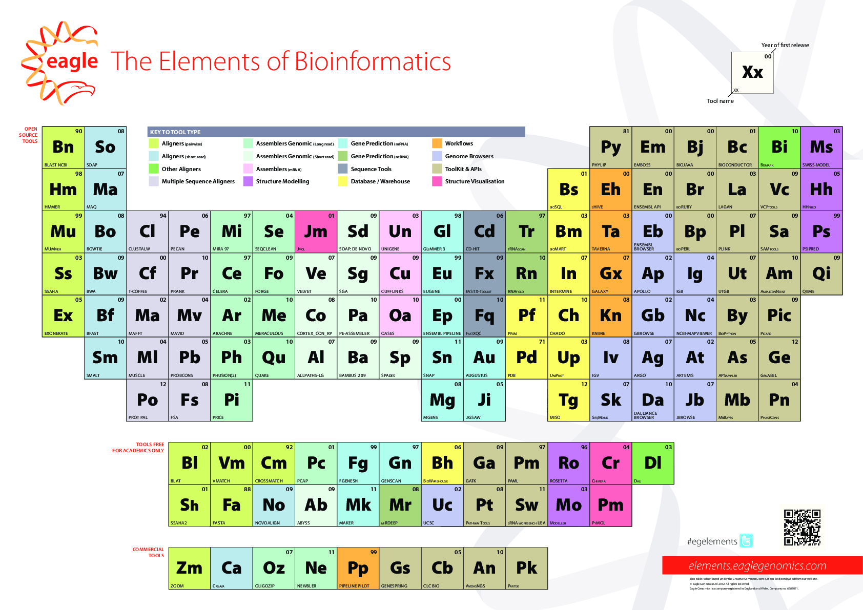
本页整理自 Eagle Genomics 发布的「生物信息学元素周期表」(The Elements of Bioinformatics),
收录了基因组学与生物信息学领域最具代表性的开源与商业工具。
这些工具贯穿从原始测序数据处理、基因组拼接、基因预测,到变异分析、结构可视化、数据库访问的完整分析流程,
是现代生命科学研究不可或缺的基础设施。
以下按功能领域分类,并注明各工具的当前维护状态(截至 2025 年)。
| 缩写 | 全名 | 简介 | 维护状态 |
|---|---|---|---|
| Bn | BLAST NCBI | 最经典的本地序列相似性搜索工具,广泛用于蛋白质和核酸数据库比对 | ✅ 活跃维护 |
| So | SOAP | 短序列比对工具,适用于 Illumina 数据的快速比对 | ⚠️ 基本停止更新 |
| Hm | HMMER | 基于隐马尔可夫模型的蛋白质序列同源搜索工具 | ✅ 活跃维护 |
| Ma | MAQ | 早期短读长比对与 SNP 调用工具 | ❌ 已停止维护 |
| 缩写 | 全名 | 简介 | 维护状态 |
|---|---|---|---|
| Mu | MUMmer | 用于完整基因组序列快速比对的系统,适合草图和完整基因组 | ✅ 活跃维护(MUMmer4) |
| Bo | Bowtie | 超快速短 DNA 序列比对工具,内存高效 | ✅ 活跃维护(Bowtie2) |
| Ss | SSAHA | 基于哈希的短序列比对工具 | ⚠️ 维护较少 |
| Bw | BWA | Burrows-Wheeler 比对工具,是目前最广泛使用的 DNA 比对软件之一 | ✅ 活跃维护 |
| 缩写 | 全名 | 简介 | 维护状态 |
|---|---|---|---|
| Cl | ClustalW | 经典多序列比对工具 | ⚠️ 维护较少(已有 Clustal Omega 替代) |
| Cf | T-COFFEE | 高精度多序列比对工具,支持结构信息辅助比对 | ✅ 活跃维护 |
| Bf | BFAST | 支持颜色空间读长的比对工具 | ❌ 已停止维护 |
| 缩写 | 全名 | 简介 | 维护状态 |
|---|---|---|---|
| Ex | EXONERATE | 灵活的序列比对工具,支持蛋白质、DNA 比对及剪接位点识别 | ⚠️ 维护较少 |
| Sm | SMALT | 短读长比对工具,适合高多态性基因组 | ❌ 已停止维护 |
| 缩写 | 全名 | 简介 | 维护状态 |
|---|---|---|---|
| Pe | PECAN | 基因组比对与拼接辅助工具 | ⚠️ 维护较少 |
| Pr | PRANK | 进化感知的多序列比对工具,考虑插入缺失的进化历史 | ✅ 活跃维护 |
| Ma | MAVID | 多基因组比对工具 | ❌ 已停止维护 |
| Mi | MIRA 97 | 多平台序列拼接工具,支持 Sanger、454、Illumina 数据 | ⚠️ 维护较少 |
| Ph | PHUSION2 | 重复序列处理优化的全基因组拼接工具 | ❌ 已停止维护 |
| Po | PROT PAL | 蛋白质序列比对工具 | ❌ 已停止维护 |
| 缩写 | 全名 | 简介 | 维护状态 |
|---|---|---|---|
| Se | SEQCLEAN | 序列清洗与质量过滤工具 | ❌ 已停止维护 |
| Fo | FORGE | 基因组拼接工具 | ❌ 已停止维护 |
| Qu | QUAKE | 基于 k-mer 的测序错误校正工具 | ❌ 已停止维护 |
| Fs | FSA | 进化感知型多序列比对工具 | ❌ 已停止维护 |
| Pi | PRICE | 迭代序列拼接工具,适合靶向序列恢复 | ⚠️ 维护较少 |
| 缩写 | 全名 | 简介 | 维护状态 |
|---|---|---|---|
| Jm | JMX | 转录组拼接相关工具 | ❌ 已停止维护 |
| Ve | VELVET | 基于 de Bruijn 图的短读长基因组拼接工具 | ⚠️ 已被 SPAdes 等替代 |
| Me | MERACULOUS | 高效的大基因组二倍体拼接工具 | ✅ 活跃维护 |
| Al | ALLPATHS-LG | 专为大型基因组设计的高质量拼接工具 | ❌ 已停止维护 |
| 缩写 | 全名 | 简介 | 维护状态 |
|---|---|---|---|
| Ce | CELERA | Celera 拼接工具,曾用于人类基因组计划 | ❌ 已停止维护 |
| Ar | ARACHNE | 全基因组鸟枪法序列拼接工具 | ❌ 已停止维护 |
| Pb | PROBCONS | 基于概率一致性的多序列比对工具 | ⚠️ 维护较少 |
| Ba | BAMBUS 209 | 基因组支架构建工具 | ❌ 已停止维护 |
| 缩写 | 全名 | 简介 | 维护状态 |
|---|---|---|---|
| Sd | SOAP de novo | 基于 de Bruijn 图的基因组拼接工具 | ⚠️ 维护较少 |
| Sg | SGA | 基于字符串图的序列拼接与分析工具 | ✅ 活跃维护 |
| Co | CORTEX CON RP | 基于 de Bruijn 图的变异检测与拼接框架 | ✅ 活跃维护 |
| Pa | PE-ASSEMBLER | 双端读长拼接工具 | ❌ 已停止维护 |
| Mg | MGENE | 基因预测工具 | ⚠️ 维护较少 |
| Ji | JIGSAW | 结合多种证据的基因预测工具 | ⚠️ 维护较少 |
| 缩写 | 全名 | 简介 | 维护状态 |
|---|---|---|---|
| Un | UNIGENE | NCBI 非冗余基因簇数据库与工具集 | ❌ NCBI 已于 2019 年停止更新 |
| Cu | CUFFLINKS | RNA-seq 转录本拼接与定量工具 | ⚠️ 已被 StringTie 等替代 |
| Oa | OASES | 基于 Velvet 的转录组从头拼接工具 | ❌ 已停止维护 |
| Sp | SPAdes | 圣彼得堡基因组拼接工具,支持多平台数据,现已成为标准拼接工具 | ✅ 活跃维护 |
| 缩写 | 全名 | 简介 | 维护状态 |
|---|---|---|---|
| Gl | GLIMMER 3 | 用于原核生物基因组的基因预测工具 | ⚠️ 维护较少 |
| Fx | FASTX-Toolkit | 用于 FASTA/FASTQ 文件预处理的命令行工具集 | ⚠️ 维护较少(已有更多替代品) |
| Eu | EUGENE | 用于真核生物基因组注释的基因预测工具 | ⚠️ 维护较少 |
| Ep | ENSEMBL PIPELINE | Ensembl 基因组注释自动化流程 | ✅ 活跃维护 |
| Sn | SNAP | 用于真核生物基因预测的隐马尔可夫模型工具 | ⚠️ 维护较少 |
| Au | AUGUSTUS | 高精度真核生物基因预测工具,支持多种物种训练模型 | ✅ 活跃维护 |
| 缩写 | 全名 | 简介 | 维护状态 |
|---|---|---|---|
| Py | PHYLIP | 经典系统发育分析软件包 | ⚠️ 维护较少(已有 IQ-TREE 等替代) |
| Bs | aoSQL | 生物信息学数据库查询相关工具 | ❌ 信息有限 |
| Tr | tRNAscan | tRNA 基因识别工具,广泛用于基因组注释 | ✅ 活跃维护(tRNAscan-SE 2.0) |
| Rn | RNA-old | RNA 序列分析工具(早期版本) | ❌ 已停止维护 |
| In | INTERMINE | 生物数据整合与查询平台 | ✅ 活跃维护 |
| Pd | PDB | 蛋白质数据库,全球最重要的蛋白质三维结构存储库 | ✅ 活跃维护 |
| Up | UniProt | 全球最全面的蛋白质序列与功能数据库 | ✅ 活跃维护 |
| Tg | MiSO | 可变剪接分析工具 | ⚠️ 维护较少 |
| 缩写 | 全名 | 简介 | 维护状态 |
|---|---|---|---|
| Em | EMBOSS | 欧洲分子生物学开放软件套件,包含大量序列分析工具 | ✅ 活跃维护 |
| Eh | eHIVE | 基于 Ensembl 的分布式流程系统 | ✅ 活跃维护 |
| En | ENSEMBL API | Ensembl 基因组数据库应用程序接口 | ✅ 活跃维护 |
| Eb | ENSEMBL BROWSER | Ensembl 基因组可视化浏览器,支持多物种基因组查看 | ✅ 活跃维护 |
| Gx | GALAXY | 开放的基于 Web 的生物信息学分析平台,无需编程基础 | ✅ 活跃维护 |
| Kn | KNIME | 数据分析与工作流平台,支持生物信息学插件 | ✅ 活跃维护 |
| Gb | GBROWSE | 通用基因组浏览器,支持本地基因组可视化 | ⚠️ 维护较少(已有 JBrowse 替代) |
| Sk | SeqMonk | 用于大规模测序数据可视化与分析的工具 | ✅ 活跃维护 |
| Nc | NCBI-MAPVIEWER | NCBI 基因组图谱可视化工具 | ⚠️ 已被 NCBI Genome Data Viewer 替代 |
| 缩写 | 全名 | 简介 | 维护状态 |
|---|---|---|---|
| Bj | BIOJAVA | 面向生物信息学的 Java 开源框架 | ✅ 活跃维护 |
| Br | aoRUBY | 生物信息学 Ruby 脚本工具 | ⚠️ 维护较少 |
| La | LAGAN | 全基因组多序列比对工具 | ❌ 已停止维护 |
| Ap | APOLLO | 基因组注释协作编辑工具 | ✅ 活跃维护(Apollo 2) |
| Ig | IGB | Integrated Genome Browser,交互式基因组可视化工具 | ✅ 活跃维护 |
| Da | DALLIANCE BROWSER | 基于网页的轻量级基因组浏览器 | ⚠️ 维护较少 |
| Ag | ARGO | 基因组拼接可视化工具 | ❌ 已停止维护 |
| Iv | IGV | Integrative Genomics Viewer,最广泛使用的基因组可视化工具之一 | ✅ 活跃维护 |
| At | ARTEMIS | 基因组序列查看与注释工具 | ✅ 活跃维护 |
| 缩写 | 全名 | 简介 | 维护状态 |
|---|---|---|---|
| Bc | BIOCONDUCTOR | R 语言生物信息学分析软件包集合,涵盖基因组、转录组、表观组分析 | ✅ 活跃维护 |
| Vc | VCFtools | VCF 格式变异文件处理与统计分析工具集 | ✅ 活跃维护 |
| Cd | CO-HIT | CD-HIT,蛋白质与核酸序列聚类工具,常用于去除冗余序列 | ✅ 活跃维护 |
| Bm | aoMART | BioMart,用于大规模生物数据整合与查询的数据挖掘工具 | ✅ 活跃维护 |
| Ta | TAVERNA | 科学工作流管理与执行平台 | ⚠️ 维护较少 |
| Pl | PLINK | 全基因组关联分析(GWAS)工具包 | ✅ 活跃维护(PLINK 2.0) |
| Sa | SAMtools | SAM/BAM 格式比对文件处理与分析标准工具 | ✅ 活跃维护 |
| Jb | JBROWSE | 下一代基于 Web 的基因组浏览器 | ✅ 活跃维护(JBrowse 2) |
| Mb | MrBayes | 贝叶斯系统发育推断工具 | ✅ 活跃维护 |
| 缩写 | 全名 | 简介 | 维护状态 |
|---|---|---|---|
| Ms | SWISS-MODEL | 蛋白质同源建模服务器,用于预测蛋白质三维结构 | ✅ 活跃维护 |
| Hh | HHpred | 蛋白质同源检测与三维结构预测服务器 | ✅ 活跃维护 |
| Ps | PSI-MED | 蛋白质结构相关分析工具 | ⚠️ 信息有限 |
| Qi | QIME | 微生物组数据分析工具(QIIME 的变体表示) | ✅ 活跃维护(QIIME 2) |
| Pic | PICARD | 基于 Java 的 NGS 数据处理工具集,常与 GATK 配合使用 | ✅ 活跃维护 |
| Ge | GenABEL | 基因组关联与表达分析 R 包 | ❌ 已停止维护 |
| Pn | PhenoCons | 表型保守性分析工具 | ⚠️ 信息有限 |
| 缩写 | 全名 | 简介 | 维护状态 |
|---|---|---|---|
| Bl | BLAT | BLAST-like 快速比对工具,由 UCSC 开发 | ✅ 活跃维护 |
| Vm | VMATCH | 大规模序列模式匹配工具 | ⚠️ 维护较少 |
| Cm | CROSSMATCH | 高度精确的序列比对程序,常用于序列修剪 | ⚠️ 维护较少 |
| Pc | PCAP | 大规模全基因组鸟枪法拼接工具 | ❌ 已停止维护 |
| Fg | FGENESH | 快速自动基因预测工具,用于真核生物基因注释 | ✅ 活跃维护(商业版) |
| Gn | GENSCAN | 经典真核生物基因结构预测工具 | ⚠️ 维护较少 |
| Bh | BioWarehouse | 生物数据仓库集成工具 | ❌ 已停止维护 |
| Ga | GATK | 基因组分析工具包,用于高通量测序数据中的变异检测 | ✅ 活跃维护 |
| Pm | PAML | 利用最大似然法进行分子进化分析的工具 | ✅ 活跃维护 |
| Ro | ROSETTA | 蛋白质结构预测与设计软件套件 | ✅ 活跃维护 |
| Cr | CHIMERA | 蛋白质三维结构可视化与分析工具 | ✅ 活跃维护(ChimeraX) |
| Dl | DALI | 蛋白质结构比对服务器 | ✅ 活跃维护 |
| Sh | SSAHA2 | 序列搜索与比对工具,适合大型基因组 | ⚠️ 维护较少 |
| Fa | FASTA | 经典序列相似性搜索工具,BLAST 的前身 | ✅ 活跃维护 |
| No | NOVOALIGN | 高精度短读长比对工具,尤其适合 SNP 分析 | ✅ 活跃维护(商业版) |
| Ab | ABYSS | 用于短读长数据的大规模基因组拼接工具 | ✅ 活跃维护 |
| Mk | MAKER | 自动化真核生物基因组注释工具 | ✅ 活跃维护 |
| Mr | seRDEEP | 深度学习辅助 RNA 编辑分析工具 | ⚠️ 信息有限 |
| Uc | UCSC | UCSC 基因组浏览器,最重要的基因组可视化平台之一 | ✅ 活跃维护 |
| Pt | PATHWAY TOOLS | 代谢通路数据库构建与分析软件 | ✅ 活跃维护 |
| Sw | sRNA workbench | 小 RNA 分析工具包 | ⚠️ 维护较少 |
| Mo | Modeller | 蛋白质同源建模工具,用于预测三维结构 | ✅ 活跃维护 |
| Pmo | PyMOL | 蛋白质三维结构可视化与分析工具,科研界标准工具之一 | ✅ 活跃维护 |
| 缩写 | 全名 | 简介 | 维护状态 |
|---|---|---|---|
| Zm | ZOOM | 高速短读长比对工具 | ⚠️ 维护较少 |
| Ca | CaLAM | 序列比对工具 | ⚠️ 信息有限 |
| Oz | OLIGOZIP | 寡核苷酸分析工具 | ⚠️ 信息有限 |
| Ne | NEWBLER | Roche 454 测序数据拼接工具 | ❌ 随 454 平台退市已停止维护 |
| Pp | PIPELINE PILOT | 拖拽式科学数据流程管理平台(Dassault Systèmes) | ✅ 活跃维护(商业版) |
| Gs | GENESPRING | 基因表达数据分析平台(Agilent) | ✅ 活跃维护(商业版) |
| Cb | CLC BIO | CLC Genomics Workbench,综合性基因组数据分析平台(QIAGEN) | ✅ 活跃维护(商业版) |
| An | AvadisNGS | NGS 数据分析平台 | ⚠️ 维护状态不明 |
| Pk | PHYML | 基于最大似然法的系统发育树构建工具 | ✅ 活跃维护 |
| 符号 | 含义 |
|---|---|
| ✅ 活跃维护 | 近年仍有版本更新,社区活跃,建议使用 |
| ⚠️ 维护较少 | 功能稳定但更新缓慢,可使用但需关注替代品 |
| ❌ 已停止维护 | 官方已不再更新,建议寻找现代替代工具 |
数据来源:Eagle Genomics · Elements of Bioinformatics | 整理时间:2025 年
minimap2 -cx asm20 --paf-no-hit CP059040.fasta adeABadeIJ_contigs.min500.fasta > asm20_all.paf
awk '$6=="*"{print $1}' asm20_all.paf
#-->contig00020
#-->contig00021
#-->contig00027
seqkit grep -v -r \
  -p "^contig00020([[:space:]]|$)" \
  -p "^contig00021([[:space:]]|$)" \
  -p "^contig00027([[:space:]]|$)" \
  adeABadeIJ_contigs.min500.fasta > adeABadeIJ_contigs.min500.no20_21_27.fasta
ragtag.py scaffold CP059040.fasta adeABadeIJ_contigs.min500.no20_21_27.fasta -o ragtag_adeABadeIJ  -C

minimap2 -cx asm20 --paf-no-hit CP059040.fasta adeIJK_contigs.min500.fasta > asm20_all.paf
awk '$6=="*"{print $1}' asm20_all.paf
#-->contig00016
seqkit grep -v -r -p "^contig00016(\s|$)" adeIJK_contigs.min500.fasta > adeIJK_contigs.min500.no16.fasta
ragtag.py scaffold CP059040.fasta adeIJK_contigs.min500.no16.fasta -o ragtag_adeIJK  -C

minimap2 -cx asm20 --paf-no-hit CP059040.fasta A6WT_contigs.min500.fasta > asm20_all.paf
awk '$6=="*"{print $1}' asm20_all.paf
#-->contig00016
seqkit grep -v -r -p "^contig00016(\s|$)" A6WT_contigs.min500.fasta > A6WT_contigs.min500.no16.fasta
ragtag.py scaffold CP059040.fasta A6WT_contigs.min500.no16.fasta -o ragtag_A6WT  -C
这说明的是:
ragtag.scaffold.confidence.txt 里列出的并不是“所有能被 minimap2 比对上的 contig”,而是“最终被 RagTag 成功放置到 scaffold/chromosome 里的 contig”。
也就是说,RagTag 的流程不是“只要能比对上就一定放进去”,而是会经过几步筛选:
再按一些条件过滤比对结果,比如:
-f)-q)然后计算 3 个置信度:
grouping_confidencelocation_confidenceorientation_confidence所以你的情况可以这样理解:
ragtag.scaffold.confidence.txt 里只看到 15 个你贴出来的这 15 个 contig 都是通过阈值的。 例如:
-i = 0.2-a = 0.0-s = 0.0你这个 contig00002 的 location_confidence = 0.1338,虽然不高,但仍然 大于 0.0,所以默认情况下还是能保留。
通常有两类原因:
例如:
这种情况下,RagTag 会认为这些 contig 不是独立的 scaffold 单元,于是不会把它们单独放进最终 chromosome。
这也是为什么:
“能比对上” ≠ “一定能被 RagTag 放进最终染色体 scaffold”
先把 21 个有比对的 contig 和最终 15 个被放置的 contig 做比较:
cut -f1 asm20.paf | sort -u > mapped21.txt
cut -f1 ragtag_output/ragtag.scaffold.confidence.txt | sort -u > placed15.txt
comm -23 mapped21.txt placed15.txt > missing6.txt
cat missing6.txt
这会得到那 6 个“有比对但没进入最终 scaffold”的 contig。
建议你开 debug 模式重新跑一次 RagTag:
ragtag.py scaffold CP046654.fasta A6WT_contigs.min500.fasta \
  -o ragtag_debug \
  -w \
  --debug \
  --mm2-params "-x asm20 -t 8"
然后检查这 6 个 contig 在 debug 文件里的情况:
grep -F -f missing6.txt ragtag_debug/ragtag.scaffold.debug.query.info.txt判断方法:
如果某个 contig 在 debug.query.info.txt 里都没有出现
-f 太高、-q 太高如果它出现在 debug.query.info.txt,但不在 confidence.txt
常见原因:
可以先试一个更宽松的参数组合:
ragtag.py scaffold CP046654.fasta A6WT_contigs.min500.fasta \
  -o ragtag_relaxed \
  -w \
  --debug \
  -f 200 \
  -q 0 \
  -i 0.0 \
  -a 0.0 \
  -s 0.0 \
  -d 200000 \
  --mm2-params "-x asm20 -t 8"
这会放宽:
-f 200:降低最小唯一比对长度-q 0:允许更低的 MAPQ-i 0.0:不限制 grouping confidence-a 0.0:不限制 location confidence-s 0.0:不限制 orientation confidence-x asm20:允许更高序列差异-d 200000:允许更远距离的 alignment merge即使你把参数放宽,也不一定能把 21 个 contig 全都放进最终 chromosome。
因为如果那 6 个 contig 是:
那么 RagTag 不放它们进去,反而是为了避免错误拼接。
换句话说:
不是参数不够宽松,而是 RagTag 认为这些 contig 不适合被独立放进最终 chromosome scaffold。
你可以加 -C:
ragtag.py scaffold CP046654.fasta A6WT_contigs.min500.fasta -C这样做的效果是:
chr0注意:
-C 不是把它们强行放进主染色体,而是把未放置 contig 收集到一个额外序列里。
你的结果说明:
其余 6 个 contig 很可能:
所以:
confidence.txt 里的 15 个,不代表只有这 15 个能比对;而是只有这 15 个最终被 RagTag 接受并用于 scaffold。
如果你愿意,我也可以继续帮你把这段整理成一版更简洁的中文操作指南。
Not quite.
What your output shows is:
mapped 22 sequences. That line should not be read as “22 contigs had accepted alignments in the PAF output.” (lh3.github.io)cut -f1 ${p}.paf | sort -u | wc -l counted 21 unique query names in the PAF file for asm5, asm10, and asm20. Since PAF normally contains alignment records, and minimap2 only includes unmapped queries in PAF if you add --paf-no-hit, the most likely interpretation is that 21 contigs had at least one reported alignment and 1 contig had no reported hit. (lh3.github.io)So the practical answer is:
No, these results do not mean all 22 contigs mapped. They suggest that 21/22 contigs produced at least one alignment in the PAF, and 1 contig did not, for all three presets. (lh3.github.io)
Also, “has at least one minimap2 alignment” is still not the same as “can be scaffolded by RagTag.” RagTag applies extra filters after alignment, including minimum unique alignment length (-f), minimum MAPQ (-q), and confidence thresholds such as grouping confidence (-i). A contig can therefore appear in the PAF but still remain unplaced by RagTag. (lh3.github.io)
To identify the missing contig exactly, run:
grep '^>' A6WT_contigs.min500.fasta | sed 's/^>//' | cut -d' ' -f1 | sort > all_contigs.txt
cut -f1 asm20.paf | sort -u > mapped_contigs.txt
comm -23 all_contigs.txt mapped_contigs.txt
Or rerun minimap2 with explicit no-hit output:
#!!!!!!!!!!! IMPORTANT: OUTPUT unmapped PAF records !!!!!!!!!!
#In the A6WT example, the contigs > 500nt has 22 records, 21 can mapped on the reference, only 15 个 contig 被 RagTag 真正放进最终 scaffold. I want to know which is not mapped, it should be plasmids --> contig00016.
minimap2 -cx asm20 --paf-no-hit CP046654.fasta A6WT_contigs.min500.fasta > asm20_all.paf
awk '$6=="*"{print $1}' asm20_all.paf
# Then delete the record contig00016, merge all contigs to a chrom sequence for submission
ragtag.py scaffold CP046654.fasta A6WT_contigs.min500.fasta -C
In that second command, minimap2 marks unmapped PAF records with * in the reference-name field. (lh3.github.io)
So your current result is actually encouraging: all three presets recover the same 21 contigs, and the remaining disagreement with RagTag is probably due more to RagTag filtering/scaffolding criteria than to minimap2 failing broadly. (lh3.github.io)
Yes — the first thing to relax is the minimap2 preset inside RagTag.
RagTag scaffold uses whole-genome alignments and defaults to --mm2-params '-x asm5'. That default is relatively strict for very closely related assemblies; minimap2 documents asm5 for average divergence not much higher than about 0.1%, while asm10 is for around 1% divergence and asm20 for several percent. RagTag then further filters alignments by unique alignment length (-f, default 1000), MAPQ (-q, default 10), and grouping confidence (-i, default 0.2). (GitHub)
A good first relaxed run is:
ragtag.py scaffold ref.fa query.fa \
  -o ragtag_asm10 \
  -w \
  -f 500 \
  -q 1 \
  -i 0.1 \
  -d 200000 \
  --mm2-params "-x asm10 -t 8"
A more permissive run is:
ragtag.py scaffold ref.fa query.fa \
  -o ragtag_asm20 \
  -w \
  -f 200 \
  -q 0 \
  -i 0.05 \
  -d 200000 \
  --mm2-params "-x asm20 -t 8"
Why these help:
-x asm10 or -x asm20 makes the assembly-to-reference aligner more tolerant of divergence. (lh3.github.io)-q accepts lower-MAPQ alignments that RagTag would otherwise discard. (GitHub)-f allows alignments with less unique anchor length to be considered. (GitHub)-d lets RagTag merge syntenic alignment blocks that are farther apart on the reference. RagTag’s paper says nearby alignments within -d are merged, with the default at 100 kb. (GitHub)-i makes RagTag keep contigs with more ambiguous chromosome assignment; RagTag excludes sequences below the confidence thresholds set by -i, -a, and -s. (GitHub)The main reason BLASTn and RagTag can disagree is that this is not just “does it hit somewhere?”. BLASTn can show local similarity, but RagTag needs filtered whole-genome alignments that are sufficiently unique and confident for grouping, ordering, and orienting contigs. If a contig maps to repeats, IS elements, rRNA operons, plasmid fragments, or multiple places equally well, BLASTn may still show hits while RagTag leaves it unplaced. That is consistent with RagTag’s unique-anchor filtering and confidence scoring. (GitHub)
Before scaffolding, I would test the minimap2 presets directly:
for p in asm5 asm10 asm20; do
  minimap2 -cx $p ref.fa query.fa > ${p}.paf
  printf "%s\t" "$p"
  cut -f1 ${p}.paf | sort -u | wc -l
done
That is useful because RagTag uses minimap2 by default, so this tells you whether the loss happens at the alignment stage or later during RagTag filtering. (GitHub)
One important caution: making RagTag too permissive can produce false joins. If your contigs are plasmid-derived, mobile-element-rich, or genuinely absent from the reference, relaxing parameters may force incorrect scaffolding rather than solve the problem. RagTag’s own paper notes that repetitive or ambiguous alignments can mislead scaffolding, and contigs with no acceptable filtered alignments are output as unplaced. ([PMC][3])
If you want, paste your exact ragtag.py scaffold command plus the number of contigs in asm5, asm10, and asm20, and I’ll tune a safer final command for your dataset.
[3]: https://pmc.ncbi.nlm.nih.gov/articles/PMC9753292/ ” Automated assembly scaffolding using RagTag elevates a new tomato system for high-throughput genome editing – PMC “
Here is a tightened version with citations placed at the ends of sentences. The references below use the primary papers for Trimmomatic, SPAdes, Multi-CSAR, BLAST, the NCBI nt resource, and PGAP. (PubMed)
Paired-end reads were quality filtered and trimmed using Trimmomatic v0.39 1. De novo genome assemblies were generated with SPAdes v3.15.5 2. For the A. baumannii ΔadeABΔadeIJ mutant, the assembly comprised 29 contigs >500 bp, whereas the ΔadeIJK mutant and the wild-type strain each yielded 22 contigs. These contigs were subsequently scaffolded with Multi-CSAR v1.1 3, which incorporated 22, 18, and 17 contigs into chromosomal scaffolds for ΔadeABΔadeIJ, ΔadeIJK, and the wild-type strain, respectively. The remaining unplaced contigs (ΔadeABΔadeIJ, n = 7; ΔadeIJK, n = 4; wild type, n = 5) showed similarity to plasmid sequences in BLASTn searches 4 against the NCBI nucleotide (nt) database 5, suggesting that they are likely of extrachromosomal origin. Genome annotation was performed using the NCBI Prokaryotic Genome Annotation Pipeline (PGAP) 6.
References
One stylistic improvement I’d still recommend is replacing “wild-type” with “wild type” in the parenthetical count to match standard prose formatting unless your journal prefers the hyphenated form consistently.
Based on the BLAST results you provided, I can confirm that all 7 of the unplaced contigs (contig00020, contig00021, contig00022, contig00025, contig00026, contig00027, and contig00028) are indeed plasmid sequences.
Here is a breakdown of each contig, its likely plasmid type, and the supporting evidence from the BLAST hits:
contig00020
contig00021
contig00022
contig00025
contig00026
contig00027
contig00028
| Contig | Verdict | Likely Plasmid Family / Notes |
|---|---|---|
| contig00020 | Plasmid | pMAC / ATCC 19606 family (e.g., p2ATCC19606) |
| contig00021 | Plasmid | p1ATCC19606 (small, high-copy-number plasmid) |
| contig00022 | Plasmid | Plasmid sequence, also found integrated in some chromosomes. |
| contig00025 | Plasmid | Likely a plasmid-borne capsule locus, shared across Acinetobacter spp. |
| contig00026 | Plasmid | Plasmid region, shared with Acinetobacter sp. PVC-6A. |
| contig00027 | Plasmid | pMAC / pATCC19606 family. |
| contig00028 | Plasmid | Plasmid region, shared with Acinetobacter sp. PVC-6A. |
Conclusion: All seven unplaced contigs are of plasmid origin. contig00020, contig00021, and contig00027 appear to be canonical plasmids matching known A. baumannii plasmid families. contig00022, contig00025, contig00026, and contig00028 appear to be plasmid sequences that are also found integrated into chromosomes or are highly promiscuous mobile elements shared across different Acinetobacter species.
这篇稿子的核心重点,不是“基因组测序本身”,而是研究 鲍曼不动杆菌(A. baumannii)如何依靠 RND 外排泵来耐受人类用的非抗生素药物,尤其聚焦两个外排系统:AdeABC 和 AdeIJK。作者想回答的问题是:这些经典的耐药外排泵,除了排出抗生素之外,是否也能把抗抑郁药、抗精神病药、抗肿瘤药、NSAIDs 等“非抗生素”排出去,从而帮助细菌存活。
更具体地说,这篇文章的主线有四层。第一层,是证明 AdeABC 和 AdeIJK 都参与非抗生素耐受。作者构建了不同的敲除株,在 ATCC19606 和 AYE 两个背景下做药敏比较,发现删掉这些外排泵后,细菌对多种非抗生素更敏感,说明这些泵确实在帮助细菌抵抗这类药物。
第二层,是说明 AdeABC 和 AdeIJK 的底物偏好不一样,也就是“分工不同”。文中结果显示,AdeABC 更偏向外排疏水性高、极性低的分子,例如一些抗抑郁药、部分酚噻嗪类抗精神病药和 diphenhydramine;而 AdeIJK 更偏向处理极性更高、氢键能力更强的分子,比如一些抗肿瘤药、部分 NSAIDs 和其他较高极性的非抗生素。换句话说,这篇文章的一个重要贡献,是把“RND 外排泵能排非抗生素”进一步细化成“不同泵对不同化学性质分子有选择性”。
第三层,是讨论 这些非抗生素不仅是外排底物,还可能诱导耐药基因表达。作者做了 qPCR,发现不同非抗生素会以药物依赖的方式诱导 adeB 或 adeJ 的表达;其中 mitomycin C 还会同时诱导 craA,提示 AdeIJK 和 CraA 之间可能存在协同外排。也就是说,文章不只是在看“药物能不能被排出去”,还在看“药物会不会反过来刺激细菌把外排系统开得更强”。这和“非抗生素促进交叉耐药”这个大问题直接相关。
第四层,是从 化学性质和结构机制 上解释为什么 AdeABC 和 AdeIJK 会偏好不同底物。作者把药物的 XlogP、TPSA、氢键供体/受体等理化参数与表型做相关分析,又结合 AdeB / AdeJ 的分子对接,提出:AdeB 的结合口袋更偏疏水,因此更适合疏水、低极性分子;AdeJ 的口袋更偏极性、带电,更容易与高极性、能形成更多氢键的分子相互作用。 这部分是文章的“机制解释”,用来支撑前面的药敏现象。
所以,如果用中文简单概括整篇稿子的“focus”,可以说:
这篇论文主要研究鲍曼不动杆菌的 RND 外排泵 AdeABC 和 AdeIJK 如何介导对非抗生素药物的天然耐受,并进一步揭示两者在底物选择性、诱导表达和结构基础上的差异。 它想传达的中心信息是:非抗生素药物也可能被细菌识别并外排,甚至还能诱导外排泵表达,因此它们可能成为促进多重耐药和交叉耐药的选择压力。
顺便提醒你一句:从这篇稿子的结构来看,whole genome sequencing 不是论文主角,只是用来辅助验证某个突变株构建是否正确、是否存在额外突变;真正的主线仍然是 非抗生素耐受表型、外排泵表达调控、以及底物识别机制。
如果你愿意,我可以下一步直接帮你把这篇文章概括成一段适合组会汇报的中文摘要。
Not really. As the manuscript is written now, the three genomes named in 2.8 are not all clearly used in the Results.
What is clear:
So the practical answer is:
Another issue is that ANI, assembly statistics, and plasmid findings are described in Methods, but I do not see those outputs actually reported in the Results text you shared.
My hint for revision: You should either
A stronger Results sentence could be something like:
Whole-genome sequencing was primarily used to validate the ATCC19606 ΔadeIJK mutant, confirming the intended deletion, excluding additional off-target mutations, and detecting retention of an adeK fragment.
And if WT and ΔadeABΔadeIJ were also truly used, add one sentence such as:
The WT and ΔadeABΔadeIJ assemblies were used as reference genomes for comparison of deletion boundaries / plasmid content / ANI / secondary mutations.
Right now, that use is not visible in the manuscript.
One more point: the wording around ΔadeIJ, ΔadeIJK, and partial adeK deletion is a bit confusing in Results, so readers may not immediately understand which sequenced mutant is being discussed.
I can help you draft a revised version of section 2.8 and the matching Results sentence.