Protected: DNA sequencing data analysis
Enter your password to view comments.
在临床试验中进行高通量分子测量变得越来越普遍。结合机器学习的进步,这些发展为基于大数据训练的算法开辟了预测患者是否会从治疗中获益的可能性。在这里,我们介绍培训这些算法的关键概念和常见方法。
将机器学习应用于临床数据的目的是建立一个计算模型,以患者特异方式从输入变量(任何可用的人口统计,临床和分子数据)中预测目标变量(如治疗反应)。除了预测模型,这样的分析还回答了以下关键问题:
我们的重点是预测治疗反应,但这同样适用于预测其他临床变量,例如患者生存。
通常,目标变量被视为二元变量,例如,0表示未响应,1表示响应治疗。模型是以算法方式训练的,根据输入变量预测目标变量。
在训练阶段,算法使用输入变量和目标变量来建模它们之间的关系(见下图)。在训练阶段使用的任何数据都称为训练数据。模型训练后,可以仅使用输入变量来预测目标变量。重要的是,可以在验证数据上估计模型的性能,而这些数据未用于训练。
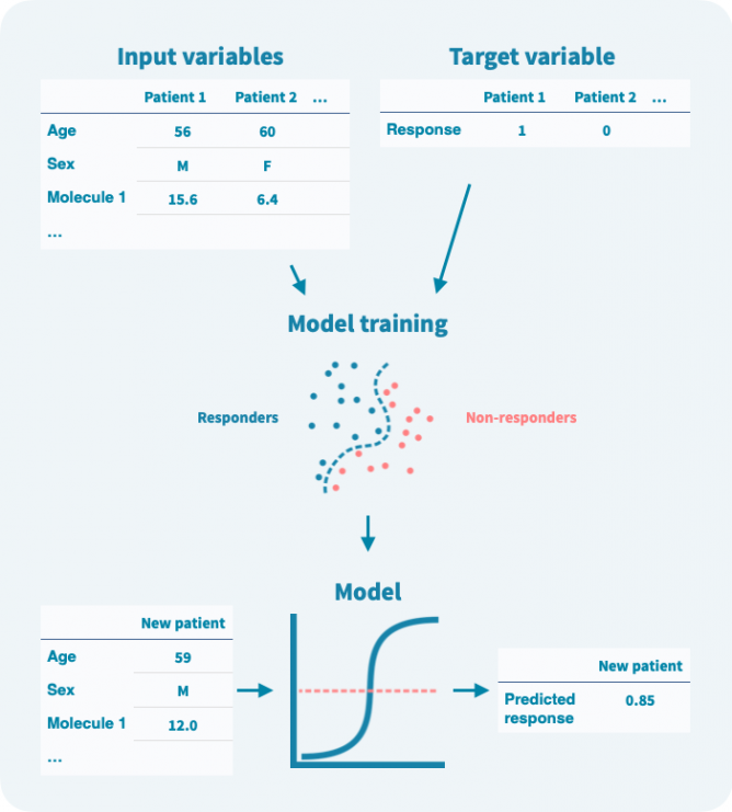
即使目标变量是二元的,模型预测通常也是概率性的——在0和1之间的数字。可以定义一个阈值来将预测二元化。设置阈值涉及灵敏度和特异性之间的权衡(参见模型验证和性能评估部分)。
输入变量可以进行预过滤以减少噪声、模型复杂度和计算量。这种预过滤称为特征选择(被认为是无信息量的变量被过滤掉,而信息量丰富的变量被选定)。此外,在训练阶段可以通过正则化来限制模型的复杂度,或者逐步惩罚算法增加模型的复杂度。限制模型的复杂度旨在避免过度拟合,即模型过度学习了训练数据:它在训练数据上表现准确,但在验证数据上表现不佳。
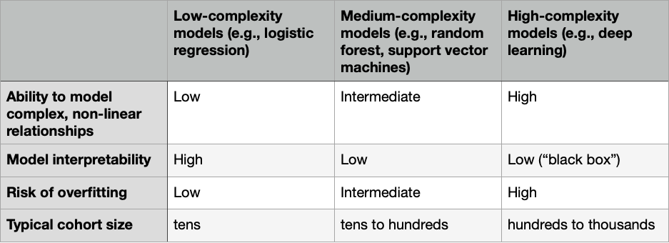
用于从输入变量预测目标变量的计算模型具有多种形式,但模型选择中涉及的主要权衡与模型的复杂性有关。更复杂的模型可以实现更好的预测,但需要更多的数据,更难解释,并且更容易过拟合。我们可以根据其复杂性将模型类型分类如下表所示:
在量化预测模型的性能时,需要确保它不仅在训练数据上工作足够准确,而且也可能在未用于训练模型的新样本上工作。
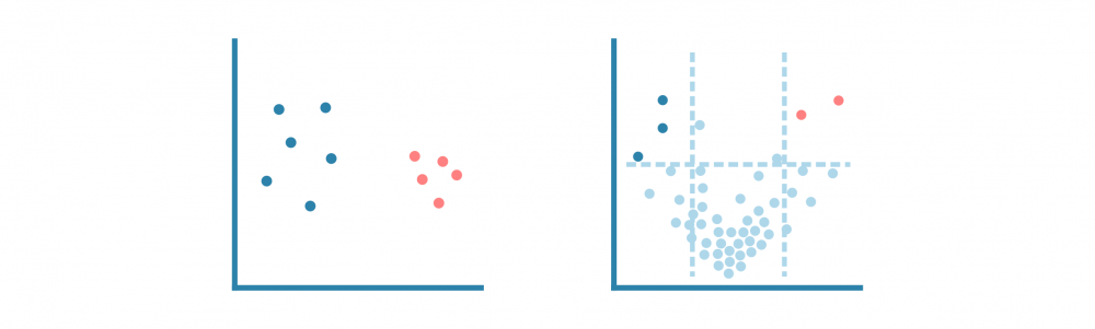
假设我们已经训练了一个模型来预测治疗反应(介于0和1之间的值),并且我们使用已知反应的十个患者的输入变量运行该模型。通过使用任何阈值对预测进行二元化,例如0.5,我们可以将十个患者的预测和已知反应制成混淆矩阵,看起来像这样:
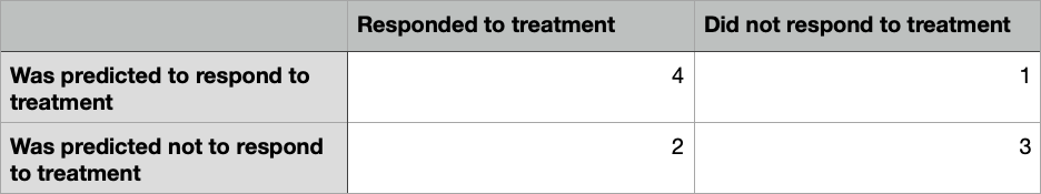
预测算法或分类器最常见的性能指标基于混淆矩阵。在上面的例子中,10名患者中有7名治疗反应被正确预测,总准确率为70%。假阳性率(FPR)为4中的1,即25%,假阴性率(FNR)为6中的2,即33%。此外,可以计算真阳性率(TPR或灵敏度)为1−FNR = 67%,真阴性率(TNR或特异度)为1−FPR = 75%。
尽管总体准确率是模型性能的简单易懂的度量方式,但问题在于它需要定义一个硬阈值来将预测二值化。一个更健壮的性能指标,它不依赖于单个阈值值,称为曲线下面积(AUC),并且是基于ROC曲线计算的。ROC曲线显示真阳性率如何取决于假阳性率(见下图)。
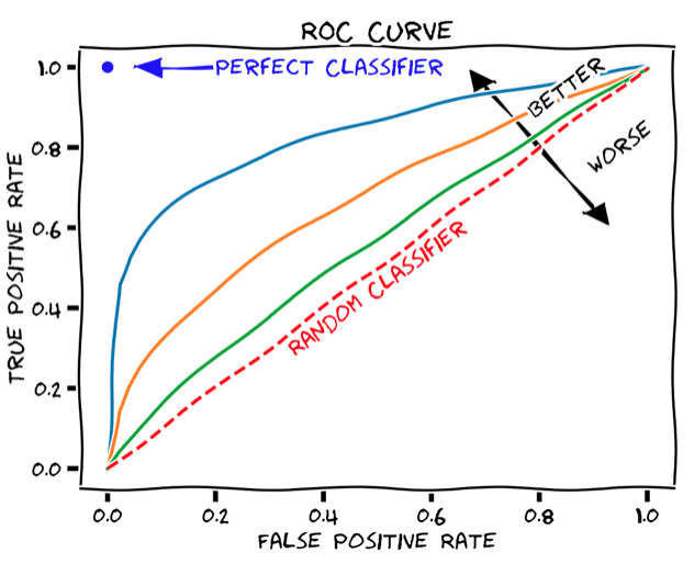
ROC曲线可以通过逐渐增加二元分类阈值从0(其中所有患者都被分类为响应者,TPR和FPR均为1,即ROC图的右上角)到1(其中所有患者都被分类为非响应者,TPR和FPR均为0,即ROC图的左下角)来产生。 AUC只是保留在ROC曲线下方的图形面积。任何分类器的AUC至少为0.5,对应于随机分类器的直线ROC曲线(上图中的虚线红线)。理想的、完美的分类器将具有最大的AUC值1。因此,现实世界的分类器的AUC值通常介于0.5和1之间。
理想情况下,应使用训练数据来训练模型,并有单独的验证队列来估计性能(最重要的是AUC),以确保模型具有可推广性。但是,对于样本数量有限的情况,通常采用交叉验证方法。在交叉验证中,模型使用(随机选择的)部分数据进行训练,并使用剩余数据进行验证,该过程重复进行,通常是使每个患者在训练中使用9次,验证模型1次(10倍交叉验证)。然后可以使用适当定义的分别训练的模型的平均值作为最终模型。
在任何实际的机器学习项目中,主要限制往往是数据量的大小。更大的样本量可以提供更好的模型,从中发现更好的生物标志物和更深入的生物学结论。将来自不同但相似的患者队列的数据(如果有)合并以训练单个模型是增加样本量的一种方式。如果存在多个系统性差异的变量(例如年龄、性别、使用的测量平台),这些变量可能会混淆:即使它们之间没有真正的关系,算法也可能将一个变量视为另一个变量的代理。在多个队列中,可以同时使用所有队列和每个队列单独进行训练模型。仔细检查模型之间的预测变量可能会揭示可能存在的混淆因素。
除了模型的预测能力外,还有其他因素决定其有用性。其中之一是其复杂性:与复杂模型相比,简单模型更快,更容易作为易于使用的工具用于研究和临床目的。另一个因素是在临床环境中量化所需生物标志物的可行性。因此,将模型训练在体液样本数据上可能比在实体组织活检中发现需要侵入性样本收集的生物标志物更有意义。
癌症治疗方案涉及疗效和副作用之间的重要权衡。为了将患者分配到最佳治疗方案,必须能够在诊断后不久预测他们的风险水平。在临床环境中生成的分子数据的增加使得预测更加准确成为可能,但是需要采用复杂的方法来训练预测算法。在我们 另外的文章 中曾經讨论过机器学习主题,现在我们专注于使用一种称为随机森林的方法来预测癌症生存。
上一次,我们介绍了机器学习的关键概念,考虑了一个简单的预测治疗反应的情况。现在,我们将更详细地了解预测算法的内部工作原理,这次是在预测生存的情况下。
生存分析通常使用Kaplan-Meier估计(用于单个预测变量或输入变量)和Cox回归(用于少量预测变量)。然而,这些方法不容易适用于具有复杂的非线性预测变量之间的高维数据(即基因组测量)。机器学习正是为这种问题而设计的解决方案。
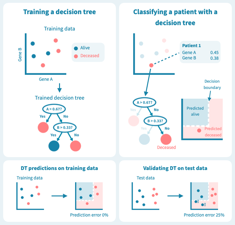
一种常见的适用于生存分析的机器学习算法称为随机森林。为了理解随机森林的工作原理,让我们首先考虑一个它所基于的更简单的算法:决策树。
下图显示了决策树在一组六个患者(三个仍然存活,三个在诊断后5年去世)上进行训练的玩具示例。使用仅来自原发肿瘤活检的两个基因的表达水平,训练后的树能够完美地分离两组患者。然而,树在测试数据上的表现——8个新的患者,这些患者未在模型训练中使用——更差,有两个患者被错分类。这描绘了机器学习中的一个核心挑战:预测模型在训练数据上可能表现非常好,但在未见过的测试数据上表现很差。过度拟合或者训练数据集过于偏斜或太小,可能导致泛化能力差。
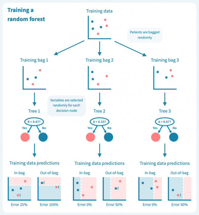
过拟合是决策树的已知问题,随机森林便应运而生,以解决这个问题。随机森林由多个决策树组成,这些树是通过对训练数据(例如患者)和预测变量(基因)进行随机子抽样而训练的。这导致了一组具有偏差但各有特点的决策树。随机森林的预测是其个别树的预测的组合(例如多数投票)。因此,随机森林是一种集成分类器,也是一种众包算法。这种方法有效地减少了个别决策树的过拟合问题。
下面的图示展示了一个随机森林(仅由三棵小树组成)在我们的玩具数据上训练的情况。每棵树都使用完整训练集(一个包)的随机样本进行训练,每棵树的每个决策节点由随机选择的基因定义。虽然树在其包中的患者表现良好(特定于树的训练数据),但它们在包外患者身上表现不佳。显然,限制在训练树时使用数据会降低其性能,这不应让我们感到惊讶!
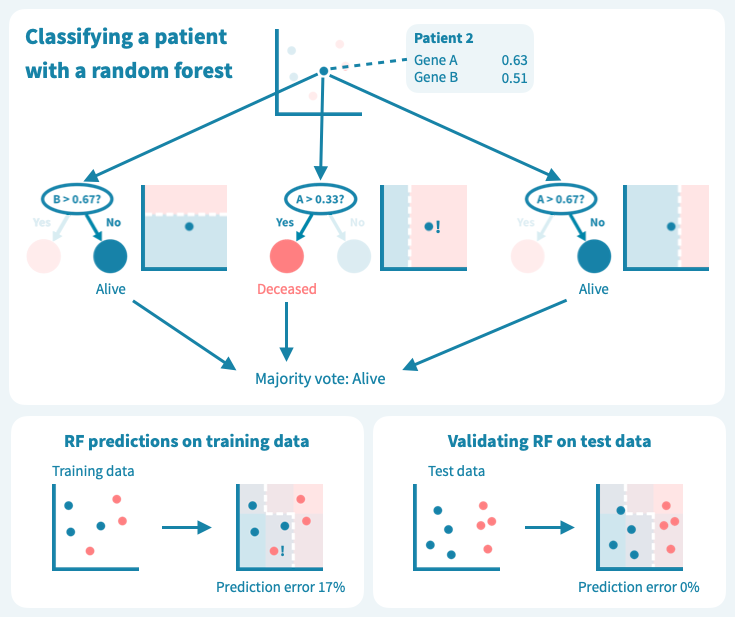
然而,这些树的组合预测在测试数据上的表现却很好——事实上,比第一个例子中的简单决策树模型要好。下面的图示展示了每个决策树如何为随机森林的集成预测做出贡献,从而在由预测变量或输入变量定义的空间中形成一个组合决策边界。
虽然我们上面的例子数据包含的患者和测量值比任何真实世界的预测问题所需的要少,但它使我们了解了算法如何基于输入变量(基因表达值)推导目标变量(例如生存状态)的预测,以及如何通过机器学习算法设计来应对泛化能力的挑战和如何对抗过拟合。
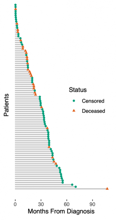
展示真实世界数据的生存预测之前,我们必须承认我们玩具数据中的另一个简化。我们假设一个简单的死亡或生存分类任务。实际上,生存数据更加复杂:患者要么死亡,要么被审查。被审查的患者按照最后一次随访仍然活着,之后他们可能很快死亡,也可能过着幸福的生活——但我们不知道。这种所谓的right-censoring是一种缺失的形式,任何生存分析都必须考虑到这一点。右图说明了生存数据:从诊断到死亡或最后一次随访的时间是已知的,而在最后一次随访时仍然存活的患者被认为是被审查的。
一种适应于生存预测的随机森林(RSF)——随机生存森林,应用于这种类型的数据。它不是将患者分类为死亡或生存,而是旨在根据其估计的风险分层患者。因此,这种模型的预测不是二元分类,而是连续的风险评分。
由于模型输出(预测)是连续的风险评分而不是易于验证的死亡或生存类别,如何评估模型的性能?一个好的答案是c指数或一致性指数。 c指数计算为具有更高预测风险的患者对中实际死亡的比例。低预测风险的患者对不能评估一致性的患者对被删减,这样的患者对是由于审查而必须接受的限制。 c指数为0.5对应于随机的、无用的分类器,而1表示按风险对患者排序的完美结果。这种c指数的解释可能会让你想起我们在 另一篇文章 中讨论的AUC的解释。实际上,c指数是对非二元预测问题的AUC的一般化。
评估模型性能的另一种方法是按预测风险对患者进行分组,绘制组特定的Kaplan-Meier估计量,并使用log-rank检验比较组。预测模型越好,高风险组和低风险组之间的区分就越明显。重要的是要基于测试数据而不仅仅是训练数据来评估这些性能指标。前者可能会更糟糕,但比后者更有信息量。
下图显示了使用来自癌症基因组图谱(TCGA)的公共数据,通过对肝癌患者的原发肿瘤的基因表达谱进行分层的结果。在TCGA-LIHC数据集的369名肝癌患者中,我们随机选择了80%,即269名患者,作为训练集来构建随机生存森林。其余的20%,即73名患者,被保留为测试集。在训练数据上的风险分层表现很好,c-指数为0.925,通过中位数风险进行二元分组可以产生具有明显不同生存模式和log-rank P值低于0.0001的风险组。
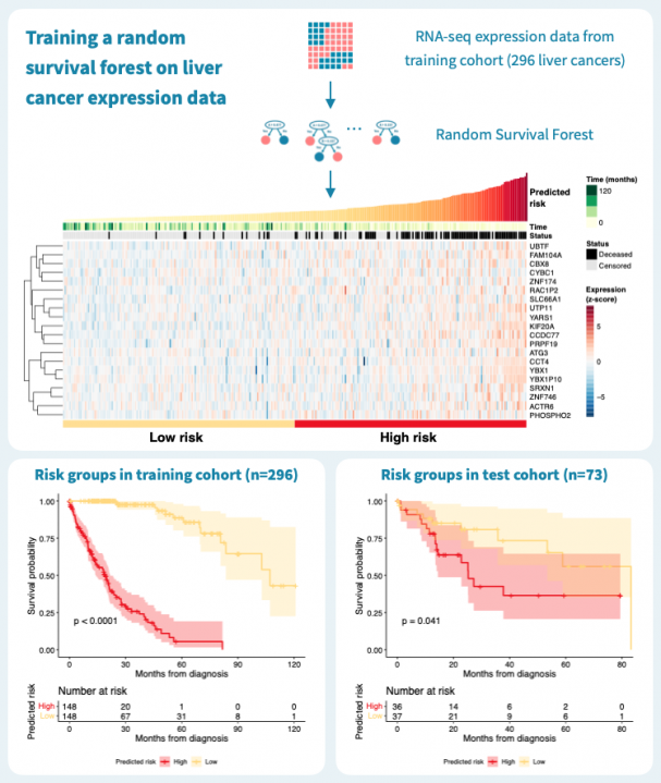
那么这个模型的推广效果如何呢?对73名患者的测试集进行的预测具有0.61的c-指数,并且二元分组的P值为0.041。性能明显优于什么都没有,但比训练数据上的性能差。这突显了使用单独的测试数据来评估模型的重要性。毕竟,训练数据上的表现对于构建模型和最终临床应用中确定的生物标志物的适用性告诉的很少。
在上面的示例中,我们只考虑了基因表达水平作为预测因子或潜在的生物标志物。机器学习模型(如随机森林)的一个重要优势是,它们允许轻松地将任何可用数据(如临床变量和突变)作为输入集成到模型中。数据越多,预测就越好,只要应用的训练和验证方案确保了泛化性!
另外 的一篇文章,介绍了机器学习的概念,并重点介绍了治疗反应预测。
我听到过许多次生物学家问这个问题(您可以将ChIP-seq替换为ATAC-seq、bisulphite-seq或任何其他 表观基因组数据 类型)。
这个问题很有意思。
生成和分析单个基于NGS的测序(如RNA-seq或ChIP-seq)的数据不像几年前那样罕见。这归功于新一代“NGS原生态”生物学家,他们在培训的早期就掌握了基本的“组学”数据分析技能,这在很大程度上消除了生物学家前往统计学系或计算机科学系的必要,向擅长编码的研究人员敲门,建议“合作”来分析他们的数据。
但是,整合不同的数据模式是另一回事,这是研究项目常常停滞的阶段。
这个想法很简单:如果您闻到、品尝和尝试一款葡萄酒,您的大脑可以整合这些多感官输入并推断出葡萄的产地,比如果只依赖一个感官更好。
那么,什么是可以采用您生成的所有可能的NGS数据并得出有洞见的多组学大脑?
我已经学会了错误答案:“这真的取决于您的研究问题。” 正确的答案是“相关性”。那是简短的答案——长的答案是“仔细分析各个数据类型,相关性,过滤,可视化,解释——迭代几次——你可能会得到一些非常好的结果!”
为了介绍这种数据整合方法,让我们假设下面可视化的实验,在几个时间点进行了RNA测序和表观基因组测序实验,以及在第一个时间点后施加了一种处理。表观基因组测序实验可以是针对一种或多种组蛋白修饰的ChIP-seq(或CUT&Tag)实验,也可以是ATAC-seq等染色质可及性实验。

(这里讨论的综合分析不需要时间序列数据;可以使用 单细胞数据 沿伪时间轨迹分析表达和表观状态,或者仅比较来自不同条件的批量实验的单一时间点数据。)
问题是,在治疗和最终改变的细胞状态之间有哪些分子机制?我们能否给出一个多步骤的描述,通过基因和基因产物网络级联的事件来重新编程细胞以适应干扰?
在转化研究的背景下,识别关键元素,如转录因子或增强子,这些元素使得细胞进入疾病状态,可以为新疗法提供可能的靶点。
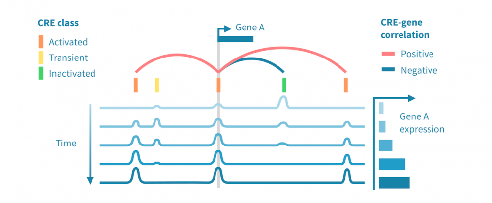
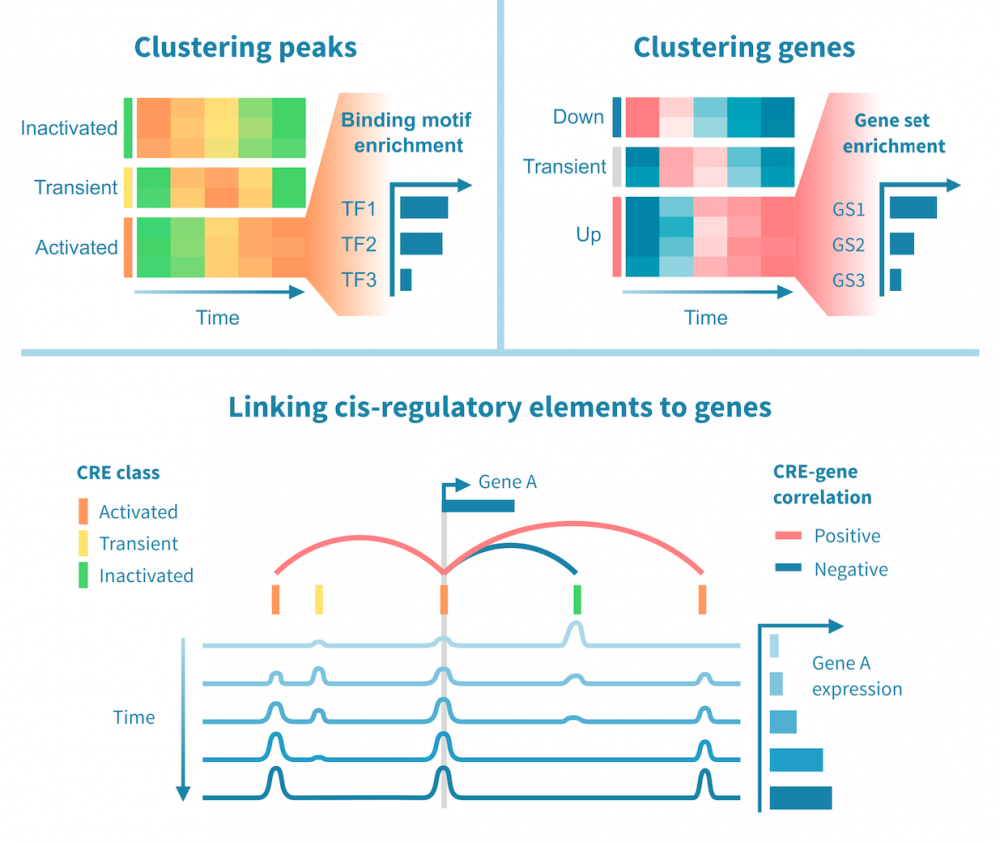
下面我们看到一个识别此类级联中活跃的顺式和反式调节路径的工作流程。它从分别处理表观基因组和转录组数据开始,并通过将每个基因的表达与其假定的顺式调节元素 (CREs) 的信号相关联,将这两种模态结合起来。然后继续通过识别驱动染色质变化的转录因子 (TFs),通过在 CREs 中识别 TF 结合基序并将 TF 的表达与这些假定的结合位点的状态相关联来确定这些 TFs。
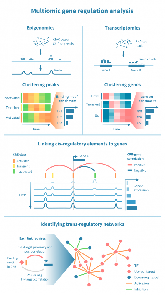
工作流程中的关键步骤包括:
上述方法描述了一个研究过程中涉及的调节程序的丰富描述。有几种方法可以进一步丰富和验证研究结果,例如:
以上我们介绍了一种整合表观基因组和基因表达数据的方法,特别是揭示cis和trans调节相互作用。了解更多关于NGS数据分析的内容:
癌症研究是生命科学中的巨头。其资金、发表的研究和生成的数据量,都超过了生物学和医学中的所有其他领域。因此,许多广泛应用于生物学的计算分析首先是为了研究癌症和突变而开发的。在这个概述中,我们将介绍癌症研究中的典型突变分析。
与任何生物医学研究一样,生物信息学常常被用于从大量的分子和临床数据中提炼新的见解。鉴于高通量测量在基础生物学和临床研究中的快速发展,生物信息学已成为癌症研究的一部分。越来越多的研究组在这个领域是由“正常”和计算生物学家组成的混合实验室。
由于湿和干生物学之间的分界正在消失,生物信息学不仅被用于从数据中提炼见解,还被用于推动研究。研究经费越来越多地授予开发计算方法而非单纯应用计算方法的癌症研究。
这里我们专注于已建立的计算方法,从突变的角度研究癌症的生物学和治疗。这些分析旨在回答以下问题:
癌症研究中的突变分析确定了肿瘤细胞DNA序列中的相关变化。除了确定单个突变外,突变模式也可以被研究,以确定突变本身的原因或癌症的克隆结构。
突变分析中的基础数据往往来自下一代DNA测序(NGS)实验。DNA测序可以应用于各种实验设置,我们在这里介绍最常见的设置。
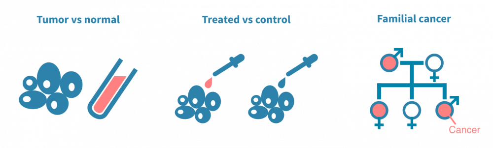
突变分析的经典设置涉及对同一患者的手术切除癌细胞和正常非癌细胞的DNA进行测序。正常细胞通常是来自血样的淋巴细胞,是一种有价值的患者特异性对照,可以与肿瘤DNA序列进行计算比较。以这种方式对多个患者进行测序,可以将突变与临床变量(如疾病亚型或治疗反应)相关联。
另一种典型实验是将经过治疗的癌细胞与未经治疗的癌细胞进行对比。在这种情况下,突变分析可以确定由治疗(如放疗)引起的突变或使癌细胞耐受治疗的突变。这种类型的实验通常依赖于动物模型或细胞系。
第三组实验旨在确定易患癌症的生殖细胞变异体。与臭名昭著的标记癌症的体细胞突变不同,生殖细胞变异体存在于个体的所有细胞中,因此可以传给后代。它们以多态性形式存在于人群中。通常,确定诱发肿瘤的遗传决定因素涉及人群规模基因分型或对患有遗传性癌症的家庭进行测序。
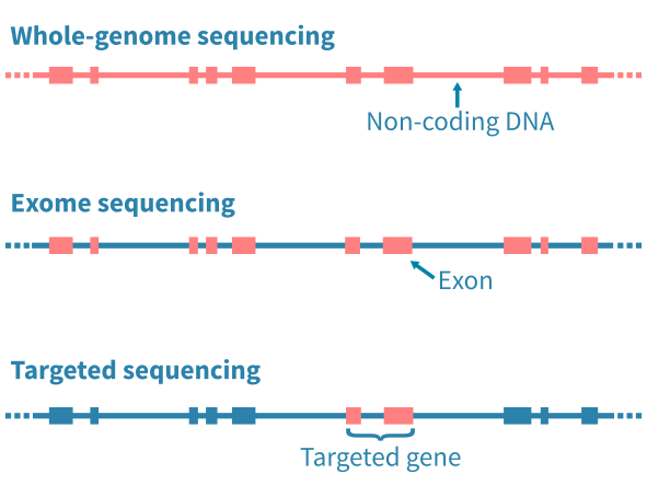
应用的DNA测序类型主要通过限制分析特定的基因组区域而影响随后的生物信息学分析。全基因组测序(WGS)能够分析基因组中的任何突变,包括广泛的非编码区域。全外显子测序(WES)限制分析基因组的编码蛋白质部分的突变。定向测序进一步限制分析到预定的基因座位 – 例如已知的癌症基因组成的panel。
DNA测序实验的原始数据进行质量控制,并与参考基因组进行比对。变异可以使用突变caller流程(mutation caller pipeline)鉴定出来。在特定调用体细胞突变时,突变caller需要将肿瘤和正常DNA-seq数据作为输入,以区分体细胞和生殖细胞突变。
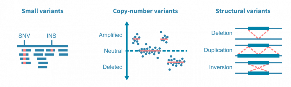
突变caller被设计用于查找特定类型的突变,例如小变异体、拷贝数变异体或结构变异体。小变异体包括一个或几个核苷酸的替换、插入和缺失。拷贝数变异体是影响更大的DNA段的扩增或删除事件。结构变异体包括更复杂的DNA改变,例如染色体间易位和DNA片段的倒位。
鉴定出的突变可以注释其变异等位基因频率、种群等位基因频率(在生殖细胞变异体的情况下)、对氨基酸序列的影响和预测的致病性。这些注释对于选择各种下游分析中相关的突变非常重要。
突变分析工作流程的关键部分是可视化鉴定的突变并将其与其他变量相关联。典型的可视化包括癌症图(瀑布图),显示多个基因在分析的患者中的突变状态,以及棒棒糖图,突出显示突变沿着变异(和编码蛋白质)基因的氨基酸序列的位置。
统计检验可用于比较不同样本组(不同癌症类型、原发性与转移性肿瘤、治疗前后等)中突变基因。突变频率、几率比和P值是此类分析中报告的典型统计量。同样,突变可以与连续变量(如患者年龄、肿瘤大小或血液生物标志物水平)相关联。
生存分析可用于将突变与临床终点(如死于癌症或复发)相关联。生存分析依赖于Kaplan-Meier估计器、Cox回归或机器学习方法。(了解更多关于生存分析的信息。)
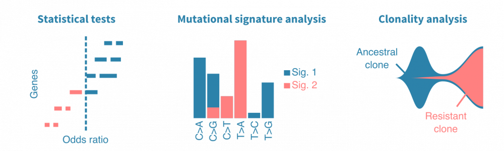
肿瘤DNA中观察到的不同类型核苷酸替换的频率 carries information on their cause。简单来说,一种致突变因子可能导致主要是T>A替换,而另一种可能导致G>C替换。比较观察到的替换频率的模式,可以定量地描述肿瘤中先前表征的突变特征。这可以揭示癌症的病因,而突变特征则是潜在的独立预后标志。
癌症是一群肿瘤细胞的动态种群,其在体内不断增殖和扩散。了解癌症如何实现增殖、逃避治疗和转移可以通过构建癌细胞家族谱来研究。当从同一患者的多个时间点或转移瘤中测序肿瘤样本时,可以研究癌症的克隆结构,并进一步将出现的女儿克隆(带有特定突变)与疾病进展事件相关联。
基于组织DNA测序的克隆分析易受数据质量和测序深度的影响。一种好的方法是首先使用全基因组或外显子组测序鉴定突变,然后对最常见的突变进行超深度靶向测序,以获得准确的突变变异等位基因估计值。
突变分析涵盖范围更广,深入程度更深,超出了我们在此简要概述的范围。如将突变数据与其他高通量数据模式集成、预测新表位、从无细胞DNA中检测突变以及解释非编码突变等主题,都需要进行进一步的介绍!
We can enable SSL on your WordPress site hosted on a Linode server either by using Let’s Encrypt with Certbot or transferring an SSL certificate from another provider (e.g., Namecheap). This guide covers both methods.
SSH into your Linode server:
ssh root@your_linode_ipInstall Certbot for your web server:
# For Ubuntu with Apache
sudo apt update
sudo apt install certbot python3-certbot-apache

# For Ubuntu with Nginx
sudo apt update
sudo apt install certbot python3-certbot-nginx
Generate the SSL certificate:
sudo certbot --apache # or --nginxFollow prompts to select your domain and enable HTTPS.
When you use Certbot, your certificates and keys are stored in /etc/letsencrypt/live/yourdomain.com/:
Certificates (fullchain.pem)
/etc/letsencrypt/live/yourdomain.com/fullchain.pemFull certificate including domain and intermediate certificates.
Private Key (privkey.pem)
/etc/letsencrypt/live/yourdomain.com/privkey.pemPrivate key associated with the certificate.
Chain of Trust (chain.pem)
/etc/letsencrypt/live/yourdomain.com/chain.pemIntermediate certificates linking your domain certificate to the root certificate.
Symlink to domain certificate (cert.pem)
/etc/letsencrypt/live/yourdomain.com/cert.pemYour domain certificate, symlinked to fullchain.pem.
The certificates and private keys should be owned by root and should be readable only by the server.
We need to adjust the permissions for any reason:
  sudo chmod 644 /etc/letsencrypt/live/yourdomain.com/*
sudo chmod 600 /etc/letsencrypt/live/yourdomain.com/privkey.pem.conf file (often located in /etc/apache2/sites-available/000-default-le-ssl.conf or a similar file) with the paths to the certificate files above.
SSLEngine on
SSLCertificateFile /etc/letsencrypt/live/yourdomain.com/cert.pem
SSLCertificateKeyFile /etc/letsencrypt/live/yourdomain.com/privkey.pem
SSLCertificateChainFile /etc/letsencrypt/live/yourdomain.com/chain.pem
For Nginx, update the ssl_certificate and ssl_certificate_key directives (typically located in /etc/nginx/sites-available/yourdomain.com).
server {
  listen 443 ssl;
  server_name yourdomain.com www.yourdomain.com;

  ssl_certificate /etc/letsencrypt/live/yourdomain.com/fullchain.pem;
  ssl_certificate_key /etc/letsencrypt/live/yourdomain.com/privkey.pem;
}Reload or restart your web server and test your site with https://yourdomain.com.
Configure certbot to auto-renew your certificates using a cron job or system timer.
sudo systemctl list-timers
sudo certbot renew --dry-run
sudo certbot certificatesWordPress needs to be updated to use HTTPS for all URLs and assets.
https:// instead of http://.You can force WordPress to always load over HTTPS by adding rules to your .htaccess file (for Apache) or nginx.conf (for Nginx).
For Apache:
Edit the .htaccess file in your WordPress root directory and add:
<IfModule mod_rewrite.c>
RewriteEngine On
RewriteCond %{HTTPS} !=on
RewriteRule ^ https://%{HTTP_HOST}%{REQUEST_URI} [L,R=301]
</IfModule>
For Nginx:
In your server block, add:
server {
    listen 80;
    server_name yourdomain.com www.yourdomain.com;
    return 301 https://$host$request_uri;
}
This ensures all HTTP traffic is redirected to HTTPS. We can also use a plugin like “WP Encryption” (chosen), “Really Simple SSL” to enforce HTTPS across your WordPress site. This plugin will automatically fix any mixed-content issues (insecure resources loaded over HTTP), ensuring that your entire site loads securely.
Follow similar steps to upload the certificate, private key, and CA bundle, then update your web server configuration as described above.
背景:耳念珠菌是一种近年来备受关注的耐药真菌,能够引起严重感染。人体的先天免疫系统,尤其是巨噬细胞(macrophages),在抵御这种病原体时发挥着重要作用。巨噬细胞通过吞噬作用(phagocytosis)来清除入侵的病菌。
MT1-MMP的作用:MT1-MMP(膜型基质金属蛋白酶1)是一种位于细胞膜上的酶,通常与细胞运动、吞噬以及细胞外基质降解相关。它需要被运输到合适的细胞膜位置才能发挥作用。
微管运输:MT1-MMP 的定位和功能依赖于细胞内部的“轨道系统”——微管(microtubules)。微管为囊泡和膜蛋白的运输提供通道。研究表明,MT1-MMP 通过微管的运输才能被有效送到巨噬细胞膜的正确位置。
与耳念珠菌吞噬的关系:当MT1-MMP能够被微管正确运输并定位在细胞膜上时,巨噬细胞的吞噬功能更高效,从而增强了对耳念珠菌的清除能力。如果微管运输受阻,MT1-MMP的定位受到影响,吞噬作用就会减弱。
结论:这项研究揭示了一个新的机制,即巨噬细胞通过微管介导的MT1-MMP运输来调控对耳念珠菌的吞噬。这为理解真菌感染的免疫防御机制提供了新的视角,也可能为开发新的治疗方法(如增强免疫清除能力)提供理论基础。
微生物合成生物学(Microbial Synthetic Biology) 是合成生物学的一个重要分支,主要利用微生物(如大肠杆菌、酵母菌、放线菌等)作为“底盘细胞”或“工程细胞”,通过基因编辑、代谢工程和合成回路设计,实现新的功能或改造其代谢路径。下面用中文详细解释:
核心概念:合成生物学的目标是像“设计机器”一样去设计和组装生物系统。微生物合成生物学就是将这一理念应用于微生物中,通过重编程它们的基因组,让它们执行我们希望的任务。
方法与工具:
应用领域:
意义:微生物合成生物学结合了生物学、工程学、信息科学与化学,既帮助人类理解生命系统的运行规律,也为可持续发展和生物经济提供了强有力的工具。
换句话说,微生物合成生物学就是 “用工程思维改造微生物,让它们为人类生产所需物质或执行特定功能”。
蛋白质组学和代谢组学揭示了生物系统的功能状态。
蛋白质和代谢物的计算分析解决了生物化学的基本问题:哪些反应发生了?正在构建什么?能量如何产生和利用?
虽然 转录组学 通常用于推断信号和代谢途径的活动,但蛋白质组学和代谢组学提供了更直接的视角,揭示了这些途径和单个反应的关键分子。
蛋白质和代谢物通常通过质谱(MS)手段进行鉴定和定量。其他方法,如依赖抗体(用于蛋白质)或核磁共振(NMR;用于代谢物)的方法提供了低通量或较少定量的数据,通常比MS更具成本效益。
除了途径分析外,患者样本的蛋白质组学和代谢组学数据特别适合于生物标志物的发现。
向下滚动以了解更多关于蛋白质组学,代谢组学和脂质组学的信息。
蛋白质组学的生物信息学分析始于识别蛋白质并量化其丰度-绝对或相对,这取决于实验。
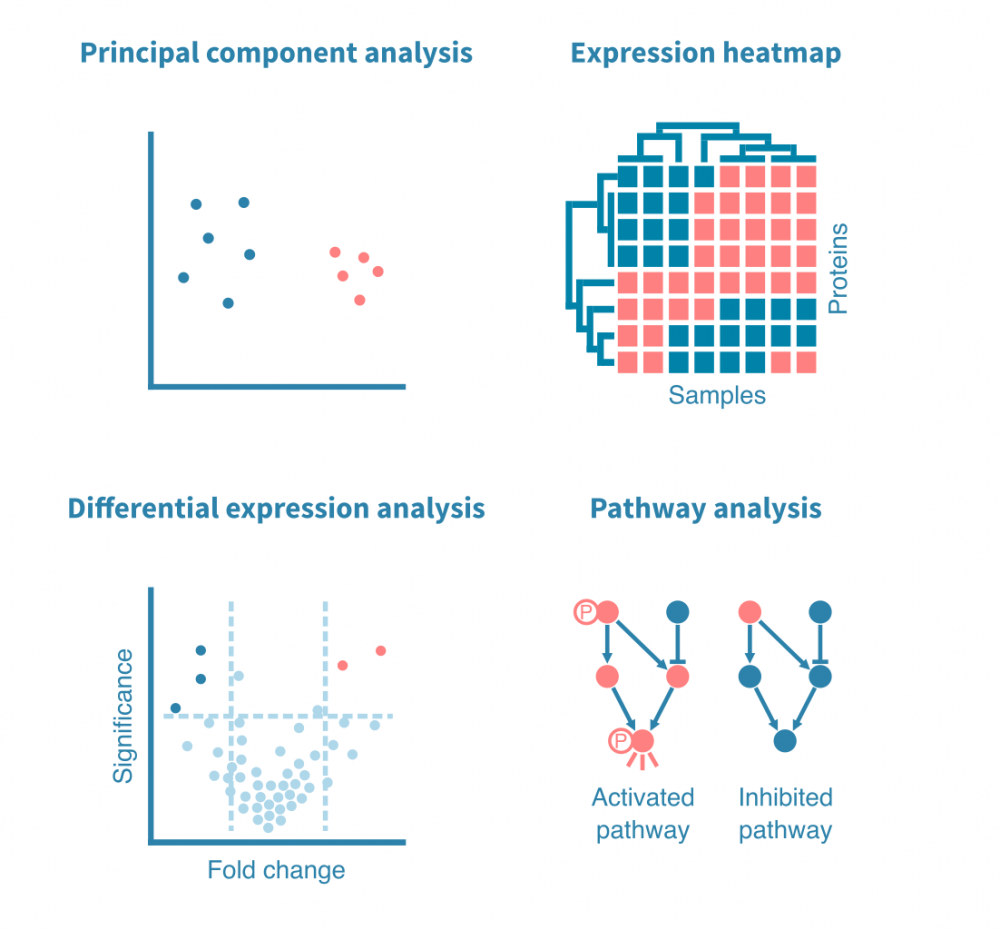
与分析任何基因表达数据一样,下一步是通过主成分分析(PCA)或类似的降维方法进行探索性分析,以研究数据集的方差和分组。
更专注的分析可能包括差异表达和途径分析,以表征样本之间的差异。
这些分析也可以针对富集了特定翻译后修饰(如磷酸化)的蛋白质进行,总蛋白质和富集子集(例如磷酸化蛋白质组)的定量数据可以并行或集成处理,以获得更详细的途径活动视图。
代谢组由参与生物体内反应的内源性和外源性小分子的几乎无限目录组成。
虽然蛋白质组学研究了这些反应的催化剂,但代谢组学关注它们的底物,中间体和产物。
与蛋白质组学类似,高通量代谢组学数据通常用于量化和研究代谢通路或识别具有临床意义的分子,例如生物标志物。因此,探索性和统计分析与蛋白质组学非常相似。
代谢组学的一个特殊案例是脂质组学,它专注于生物体内脂质分子的巨大多样性。脂质组学分析通常旨在表征脂质代谢和转运的(失)功能,特别是在代谢性疾病中。

揭示发育和疾病中基因调控的表观遗传机制。
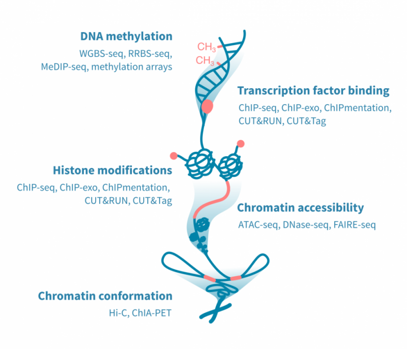
表观基因组学描述了染色质状态的微小化学修饰。DNA和相关蛋白质的表观遗传变化影响基因表达并可能导致细胞状态的改变,包括疾病。
我们分析广泛的表观基因组测序数据,以深入了解细胞内分子机制并确定疾病的生物标志物。
下面我们讨论常见的表观基因组数据类型和分析,并介绍一些我们以往的表观基因组数据分析工作。
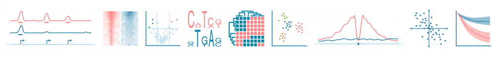
用于表观基因组分析的高通量测定方法众多,并且不断开发新的协议。最常见的表观基因组测定方法集中在DNA甲基化、DNA结合蛋白、组蛋白修饰、染色质可接近性或染色质的三维构象。
DNA甲基化: 基于亚硫酸盐处理的DNA的DNA甲基化测定可以以最高分辨率确定甲基化事件。这种测定使用下一代测序(全基因组或减少表示亚硫酸盐测序)或微阵列。另一种方法MeDIP测序,依赖于免疫沉淀,分辨率较低。
转录因子结合和组蛋白修饰: 用于确定DNA结合蛋白,如转录因子,以及组蛋白蛋白质的化学修饰的测定方法利用抗体。 ChIP-seq是最常用的方法,但已开发出具有更好分辨率的新方法。这些包括ChIP-exo、Chipmentation、CUT&RUN和CUT&Tag。
染色质可接近性: 映射开放染色质区域的黄金标准测定方法是ATAC-seq。ATAC-seq已经取代了先前的方法,例如DNase-seq和FAIRE-seq。
染色质构象: 染色质三维构象的重要性最近得到了特别的认识。染色质构象测定用于研究基因与其远端调节元素之间的物理相互作用,以及导致染色质环绕的蛋白质。Hi-C是前者的典型测定方法,而ChIA-PET可以应用于后者。
研究表观基因组对基因表达的直接影响时,通常需要在同一实验中进行RNA测序实验来补充表观基因组测量。
单细胞实验,特别是单细胞ATAC测序,越来越多地与单细胞RNA测序一起进行联合分析。这可以从同一单个细胞中获得基因表达和染色质可及性的谱。
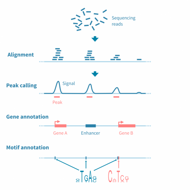
对于大多数基于测序的表观基因组数据(特别是ChIP-seq,ATAC-seq和相关实验),分析工作流程涉及识别、注释和分析峰值,或者具有感兴趣信号的基因组区域。
首先对原始测序读数进行质量控制和参考基因组的比对,之后使用可能的对照库(在ChIP-seq的情况下,预IP输入和IP与非特异性抗体)来归一化读数覆盖信号。
使用峰值caller工具识别信号中的峰值。此阶段可能需要仔细调整参数以优化用于分析的协议。
为了进行进一步的分析,使用相关信息(如读数统计和接近或重叠的特征,如基因、调控元件和结合基序)对峰值进行注释。
使用基因注释峰值可进行基因集富集分析,以进一步解释下游效应。
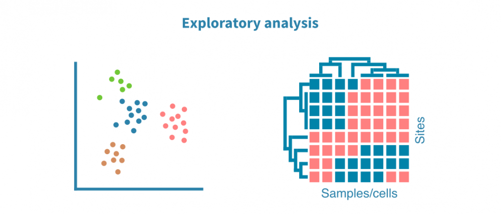
使用PCA(对于单细胞数据,使用UMAP或t-SNE算法)和热图可视化样本集中的注释峰值。这些可视化有助于优化峰值调用过程,并回答以下问题:
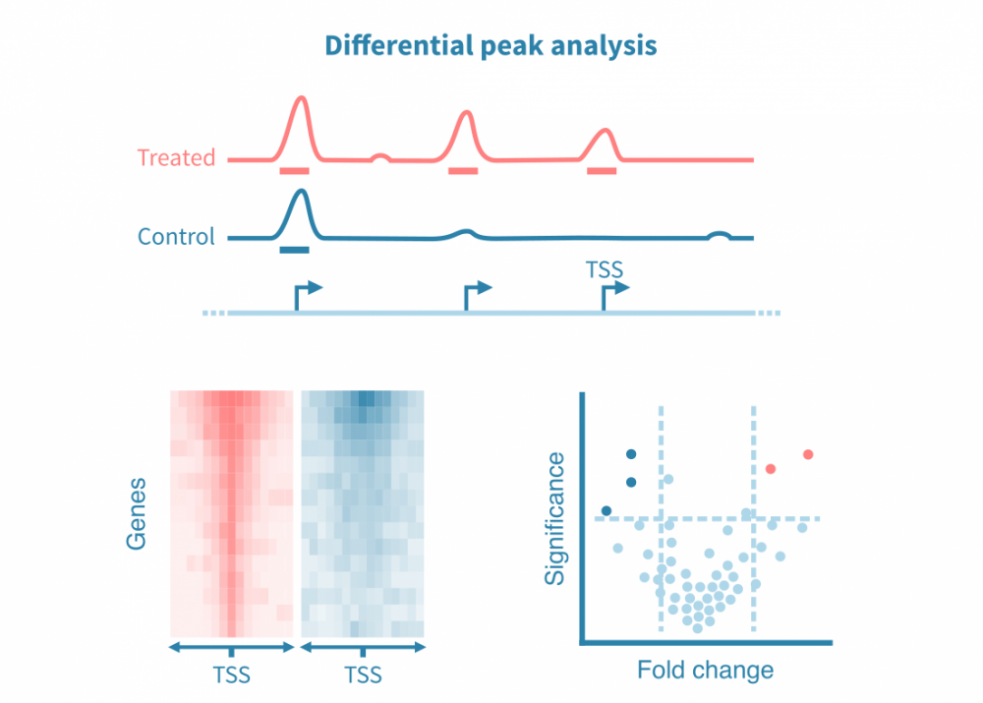
为了比较不同条件,可以对已识别的峰进行统计比较,或者更常见的是直接从各自的读数覆盖信号中调用差异峰。
类似于差异基因表达分析,差异峰分析可产生效应大小和统计显着性的估计值。这些统计数据可以可视化为火山图。
由于全基因组表观基因组测量在整个基因组中产生连续的信号,因此这些分析也可以集中于特定的感兴趣区域,例如启动子或感兴趣蛋白质的已知结合位点。密度热图用于在不同条件下可视化感兴趣位点的信号。
此外,在峰值处重叠的结合基序可以在条件之间进行统计比较,并以火山图的形式进行可视化。
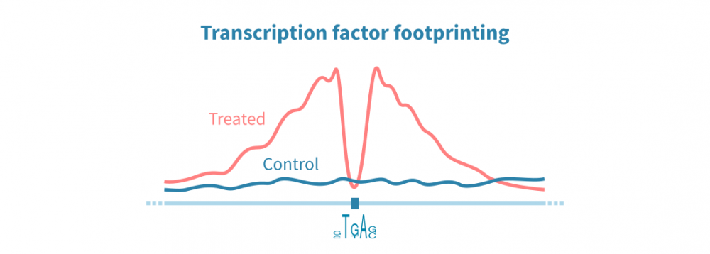
ChIP-seq和相关协议可用于在整个基因组中识别转录因子(TF)结合位点。这些检测依赖于针对感兴趣蛋白质的特异性抗体,因此这种方法可以仅识别一个TF的结合位点。另一方面,ATAC-seq数据可以通过称为TF足迹分析的方法并行识别所有DNA结合蛋白的结合位点。
在TF足迹分析中,染色质可及性信号中的窄降落被解释为蛋白质结合位点。可以间接推断TF的身份。结合RNA-seq数据,TF足迹分析可以用于以非常高通量的方式研究TF对基因表达的综合影响。
DNA甲基化数据的分析始于测序读数的质量控制和比对(或数组数据的QC和标准化),然后进行甲基化位点的调用。
检测到的甲基化位点用于识别样本之间的更大的DNA甲基化区域或差异甲基化区域(DMR)。这些区域可以类似于其他表观基因组数据中的峰值进行注释。
DNA甲基化数据的可能下游分析包括:
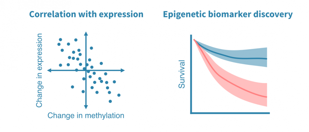
在同一样本上进行RNA-seq和表观基因组测序(如ChIP或ATAC-seq)可以进行综合分析,以研究基因调控程序的全基因组。
可以识别增强子和其靶基因之间的调节连接,以及转录因子和它们的靶基因,借助来自基因表达和调节元素表观基因组状态的证据建立。
了解更多

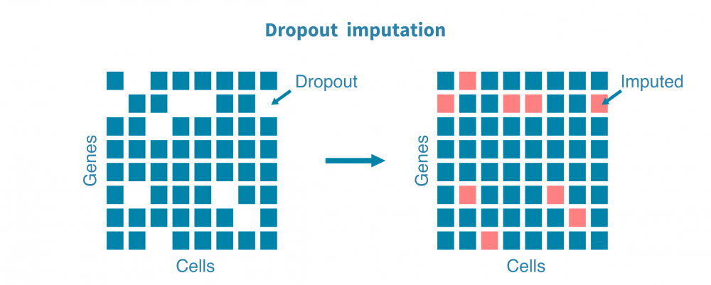
单细胞RNA测序使得细胞鉴定和研究在规模和分辨率上达到了高于批量测序的水平。
单细胞RNA测序(scRNA-seq)是分子生物学中发展和多样化最快的技术之一。研究基因表达在单个细胞水平上的能力就像之前批量RNA测序的出现一样具有变革性。
除了单细胞RNA测序,还有许多其他基于下一代测序(NGS)的检测方法已被适应于单细胞协议。这些包括基因组学、蛋白质组学和表观遗传学检测,特别是单细胞ATAC测序,通常与scRNA-seq一起进行。
平台和scRNA-seq协议在其吞吐量(细胞数)和转录本覆盖率(3’/5’标签基础 vs 全转录本)方面有所不同。我们团队在多种技术方面具有经验,如10X Genomics、Drop-Seq、BD Rhapsody系统以及CEL-Seq和Smart-Seq系列的协议。
这里我们介绍典型的单细胞分析,重点是scRNA-seq,但也涵盖了其与其他常见的单细胞检测的整合。
与任何NGS数据一样,对单细胞测序数据的分析始于质量控制和预处理。
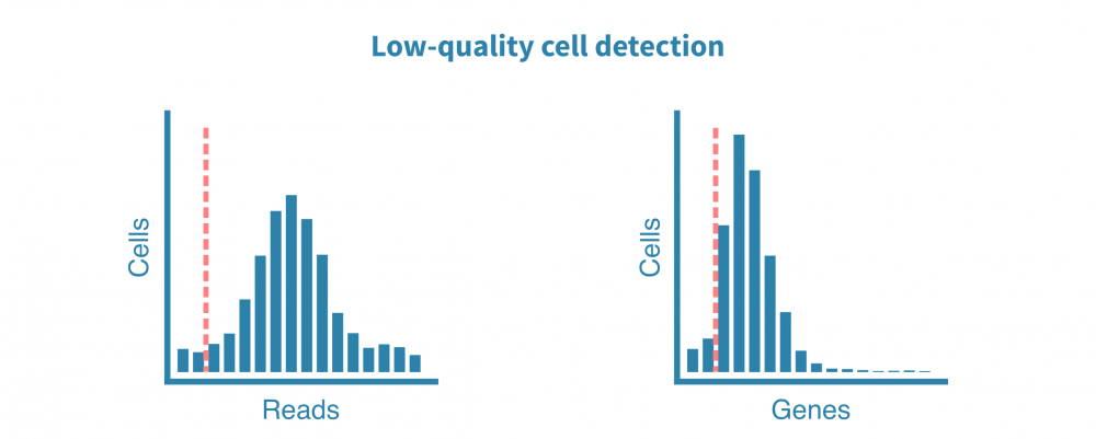
原始测序读数经过质量测试,并生成诸如细胞质量、准确性和多样性等指标。然后将读数与适当的参考基因组或转录组进行比对,并绘制和检查附加的指标,例如细胞数、每个细胞的读数、每个细胞的基因数、测序饱和度以及线粒体转录本的比例。
这些质控指标告诉我们关于文库的总体质量和样品的可用性,并使我们能够确定和去除低质量的细胞。
通常还进行进一步的预处理,以从某些下游分析中去除不需要的信号或噪声,这包括:
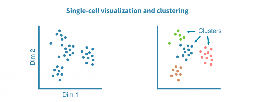
预处理的单细胞RNA测序数据被聚类以识别相似的细胞群,并使用非线性降维算法(如tSNE和UMAP)和相关性热图进行可视化,以揭示细胞异质性的一般模式。
这些可视化帮助我们回答技术问题,例如:
……以及生物学问题,例如:
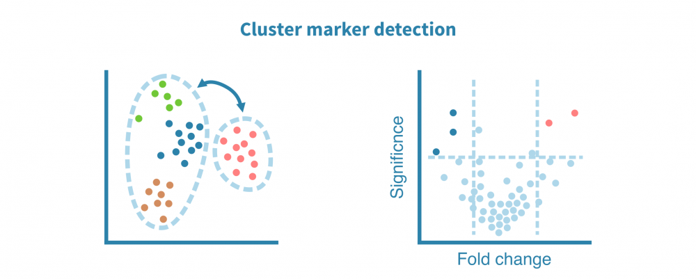
识别和表征细胞类型(以及更精细的细胞状态)是大多数单细胞项目最核心的部分。
这一切始于识别特定于每个细胞群的特征(例如基因、蛋白质、可访问区域)。这些标记由差异表达(DE)比较每个细胞群和其余细胞群而定义,产生如折叠变化和统计显着性等DE统计量。
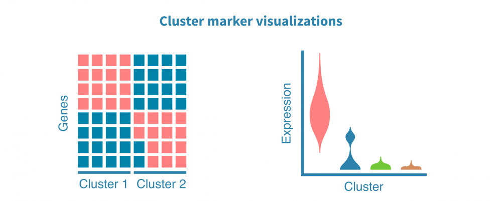
可以使用散点图、小提琴图和热图可视化细胞群标记。
标记进一步注释为生物学意义的术语,例如生物过程、信号通路或特定疾病。这些分析可能依赖于超表达分析或基因集富集分析,两者都会产生一系列富集的基因集与相关统计信息和注释。
单细胞数据集通常也与公共可用数据集集成,以利用已注释数据集或细胞图谱中的细胞类型信息。这使得将细胞标签转移至分析的数据集成为可能。
转移的细胞标签和鉴定的标记及其注释与关于细胞类型/状态标记的先前信息一起用于鉴定捕获的细胞类型。
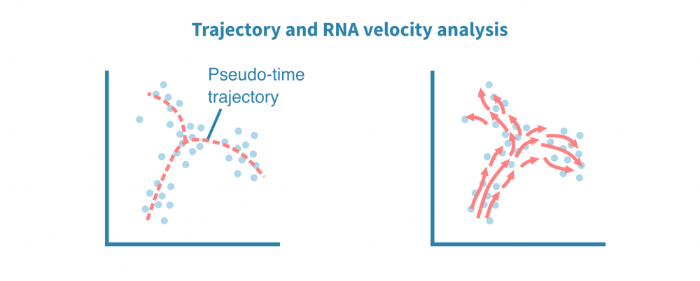
除了表征不同的细胞身份外,单细胞数据还适用于识别细胞状态渐变的连续体或轨迹。揭示这种连续体也被称为假时间分析,尽管所有细胞在同一时间点被采样,但个体细胞可能代表分化等时间过程中不同的阶段。
利用分化分支和细胞成熟轨迹的全新重建,可以探索细胞动态,勾勒细胞发育谱系,并表征沿着潜在假时间维度的细胞状态转换。
轨迹推断算法的集合可用于鲁棒地识别根和终端细胞状态、分支点和谱系。单细胞沿着确定性或概率谱系进行排序,它们的排序指示了它们在感兴趣的动态过程中的进展情况。
这种类型的分析还可以利用加工和未加工转录本的比率推断基因表达在给定细胞中是增加还是减少。将来自给定状态下所有定量基因的这些信息相结合,可以推断状态的变化方向和速度。这称为RNA速度分析。
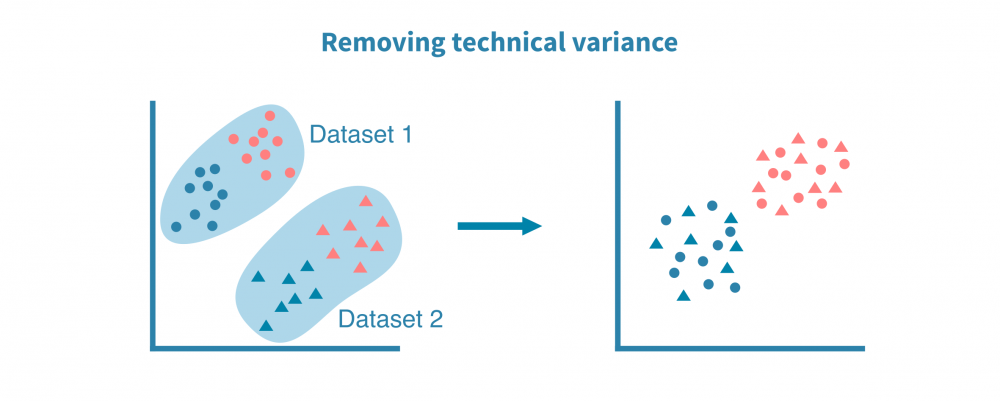
综合单细胞分析将不同的数据集,包括不同的数据类型和物种集成在一起,这使得对所研究系统中基因调控的机制有更准确和详细的细胞标记和洞察。这种分析依赖于数据集之间的共同属性或“锚点”,如匹配的特征(例如基因或同源物)或匹配的细胞。
最常见的单细胞数据集整合是来自不同来源或技术平台的scRNA-seq数据集之间的整合。使用基因作为锚点,成功的整合可以去除数据集的技术偏差同时保留生物变异。
当有关于相应组织或生物体的公共表达图谱时,整合不同的scRNA-seq数据集特别有帮助。
将单细胞RNA测序数据与单细胞ATAC-seq或单细胞甲基化数据结合起来通常依赖于匹配的细胞作为锚点(当测量来源于与10X Genomics Multiome技术中相同的细胞时)。
将表达数据与染色质可及性或甲基化数据相结合,可以更可靠地识别细胞类型,并允许量化染色质状态对各个细胞类型的表达的影响。
阅读有关整合表观遗传学和转录组学的更多信息
由于蛋白质而不是转录本是细胞功能的关键驱动因素,单细胞蛋白质组学通过更准确地估计细胞的功能状态来补充scRNA-seq实验。
单细胞蛋白质组学分析(CITE-seq,流式细胞术,质谱和质谱分析)具有不同的吞吐量(量化的蛋白质数量)并可以专门针对表面蛋白进行定向,如CITE-seq,它涉及从具有匹配scRNA-seq读数的细胞中量化表面蛋白。
表面蛋白在细胞类型鉴定中特别有用,而包含胞质蛋白则可以更好地表征通路和基因调控活动。
跨物种综合分析可确定定义不同生物之间进化和发育机制关系的细胞类型谱系。在跨物种整合中,使用共享的同源物作为锚点。
当疾病/器官在动物模型中的单细胞分辨率上得到更好的表征时,这特别有助于人类疾病/器官的研究。
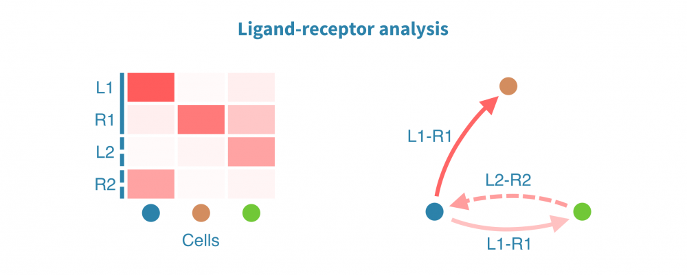
膜受体配体(LR)分析揭示了协调体内稳态、发育和其他系统级功能的细胞间相互作用。此类相互作用的变化和功能失调在仅限于个体细胞或细胞类型内部状态分析中可能不被注意到。
膜受体配体分析根据已知受体和其配体的表达量识别和量化细胞间相互作用。这些相互作用可能在组织内或组织间发生,其强度将在感兴趣的生物条件(如患者组、疾病状态和治疗)之间进行比较。
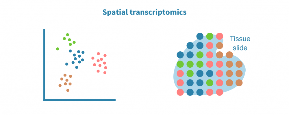
空间解析单细胞转录组学分析将表达数据与细胞在组织或器官中的位置上下文联系起来。这在研究肿瘤及其微环境等复杂实体组织中特别有用。
空间转录组分析包括空间中的细胞/点聚类、空间变量基因的识别和空间中的细胞类型解析。
保留序列化细胞的位置信息有助于准确识别细胞类型和膜受体配体相互作用。它还能够实现基因表达或染色质可及性(在scATAC-seq情况下)的空间可视化,并将基于成像的数据整合到分析中。
即使在像10X Visium这样的低分辨率分析中,多模式空间分析也有助于纠正基因表达值和补充数据缺失事件。