CRISPR-Cas9 脱靶率检测方法
问题背景
在通过电转(Electroporation)结合 CRISPR-Cas9 技术完成蛋白敲除后,评估脱靶率(off-target rate)是关键步骤。脱靶率指 Cas9 在非目标位点发生切割导致的意外变异比例。以下为回答“简单测序方式(如 pool 测序)”的建议,重点推荐多位点扩增结合 NGS(amplicon deep sequencing),并澄清 pool 测序的概念。
推荐方法:多位点扩增 + NGS(Pool 测序)
什么是 Pool 测序?
在 CRISPR 脱靶检测中,pool 测序指:
- 使用预测工具(如 CRISPOR、Cas-OFFinder)筛选潜在脱靶位点(通常几十到上百个)。
- 针对这些位点(包括目标位点)进行 PCR 扩增(片段约 200–300 bp)。
- 将所有扩增产物混合(pool)成一个测序文库,使用 NGS(如 Illumina,150 bp 读长)测序。
- 通过分析每个位点的 reads,计算 indel 率(插入/缺失比例),即脱靶率。
为什么选它?
- 简单:流程标准,实验室常用,操作直观。
- 成本低:多个位点混库测序,远低于全基因组测序。
- 结果直观:直接报告每个位点的 indel 率(如“位点A:0.5%”)。
- 可优化:加入 UMI(唯一分子标签)可减少 PCR 偏差,提高低频脱靶检测精度。
操作步骤(概念版)
- 用 CRISPOR 或 Cas-OFFinder 预测脱靶位点。
- 设计引物,针对每个位点 PCR 扩增。
- 混合扩增产物,构建 NGS 文库。
- 上机测序,分析每个位点的 indel 率。
注意事项
- 位点局限:仅覆盖预测位点,漏掉意外脱靶。需结合 GUIDE-seq 或 CIRCLE-seq 发现位点。
- 测序深度:检测 <0.1% 低频脱靶需更高深度,增加成本。
- 细胞背景:电转细胞类型可能影响脱靶谱,建议用实际样本验证。
其他方法(更全面)
如果担心漏检,可先用以下方法发现脱靶位点,再用 pool 测序定量:
- GUIDE-seq:细胞内用寡核苷酸标记双链断裂,测序定位。优点是贴近真实环境,适合安全性评估。
- CIRCLE-seq/CHANGE-seq:体外切割基因组 DNA,富集后测序,灵敏度高,适合生成候选位点清单。
Pool 测序 vs. 群体遗传学 Pool-seq
- CRISPR 的 Pool 测序:同一样本内多个位点的扩增产物混合测序,保留样本信息,适合脱靶率分析。
- 群体遗传学的 Pool-seq:混合多个个体 DNA 测序,研究群体变异,丢失个体信息,不适合单个样本的脱靶检测。
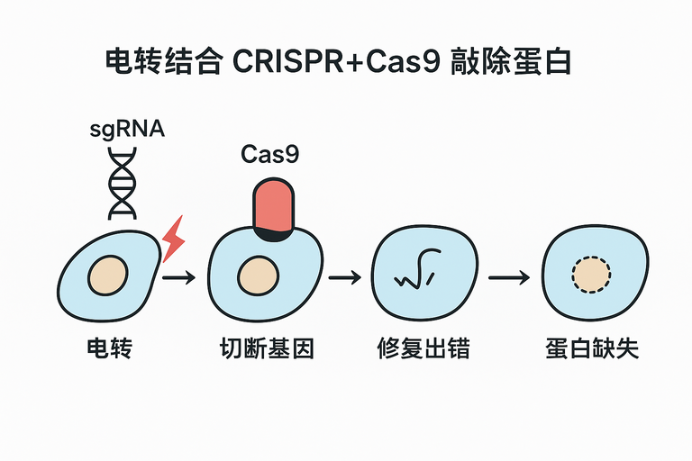
电转结合 CRISPR-Cas9 敲除原理
- 电转:通过高压电场在细胞膜上开孔,将 Cas9 蛋白和 sgRNA(或 RNP 复合物)导入细胞。
- CRISPR-Cas9:sgRNA 引导 Cas9 切割目标基因,造成双链断裂(DSB)。
- 敲除:细胞通过非同源末端连接(NHEJ)修复,常产生 indel,导致基因失活,蛋白表达消失。
结论
多位点扩增 + NGS(Pool 测序)是最简单、性价比高的脱靶率检测方法,适合快速验证预测位点的编辑率。如需更全面分析,可结合 GUIDE-seq 或 CIRCLE-seq 发现意外位点,再用 pool 测序定量。
CRISPR 脱靶检测方法对比表
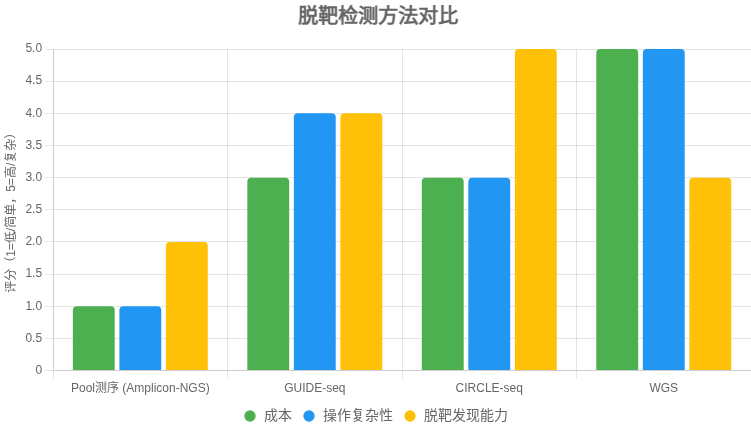
以下表格比较了 多位点扩增NGS(Amplicon-NGS,即 Pool 测序)、GUIDE-seq、CIRCLE-seq 和 全基因组测序(WGS) 在检测 CRISPR-Cas9 脱靶率时的特点,供快速选择适合方法。
| 方法 | 原理 | 优点 | 局限 | 适用场景 |
|---|---|---|---|---|
| Amplicon-NGS (Pool 测序) | 针对预测位点 PCR 扩增,混合建库,NGS 测序计算 indel 率 | – 成本低 – 操作简单,流程成熟 – 结果直观(位点 indel%) |
– 仅限预测位点 – 无法发现意外脱靶 – 低频脱靶需高测序深度 |
快速验证已知位点的脱靶率;常规研究 |
| GUIDE-seq | 细胞内用寡核苷酸标记 Cas9 双链断裂,全基因组测序定位 | – 贴近真实细胞环境 – 能发现意外脱靶 – 对低频位点较敏感 |
– 实验较复杂 – 某些细胞类型效率低 |
安全性评估;需全面发现脱靶的研究 |
| CIRCLE-seq | 体外基因组 DNA 环化,暴露 Cas9 切割,富集后测序 | – 灵敏度高 – 操作较 GUIDE-seq 简便 – 易发现低频/意外位点 |
– 体外体系,可能与细胞内偏差 – 需细胞样本验证 |
生成广谱候选位点清单,结合验证 |
| WGS | 高深度全基因组测序,观察全局变异 | – 覆盖全面 | – 成本高 – 对低频脱靶敏感度低 – 数据分析复杂 |
临床级严谨需求;补充验证 |
决策建议
- 简单需求:选 Amplicon-NGS,快速定量已知位点脱靶率。
- 全面需求:先用 GUIDE-seq 或 CIRCLE-seq 发现位点,再用 Amplicon-NGS 验证和定量。
- 高严谨性:WGS 作为补充,但成本较高。
回答:CRISPR-Cas9 敲除后脱靶率检测的简单测序方法
关于用电转结合CRISPR-Cas9敲除蛋白后,想知道脱靶率的简单测序方法,我推荐用多位点扩增结合NGS(amplicon deep sequencing),也就是您提到的“pool测序”。下面我简单说明怎么做,以及为什么它简单有效:
1. “Pool测序”是什么?
在这里,pool测序指的是:
- 先用工具(如 CRISPOR、Cas-OFFinder)预测 Cas9 可能切错的脱靶位点(通常几十到上百个)。
- 对这些位点(包括目标位点)做 PCR扩增,每个位点扩增出 200–300 bp 的片段。
- 把所有扩增产物混合(pool)成一个测序文库,上机测序(比如 Illumina,150 bp 读长就够)。
- 测序后,通过分析每个位点的 reads,计算 indel率(插入/缺失比例),这就是脱靶率。
2. 为什么选它?
- 简单:实验流程成熟,很多实验室都用这套方法,操作像“套公式”一样直观。
- 省钱:几十个位点混在一个文库里测,成本远低于全基因组测序。
- 结果直观:直接告诉你每个位点的脱靶率(比如“位点A:0.5% indel”)。
- 可优化:加 UMI(唯一分子标签)能减少 PCR 偏差,检测低频脱靶更准。
3. 注意事项
- 位点选择:脱靶率分析只覆盖你预测的位点。如果担心漏掉意外脱靶,可以先用 GUIDE-seq 或 CIRCLE-seq 找候选位点。
- 测序深度:想看 0.1% 以下的低频脱靶,得增加测序深度,稍微多花点成本。
- 细胞背景:电转的细胞类型可能影响脱靶谱,建议用你的实际样本测。
4. 简单操作步骤(概念版)
- 用软件预测脱靶位点(几十到上百个)。
- 设计引物,针对每个位点 PCR 扩增。
- 把扩增产物混在一起,建 NGS 文库。
- 上机测序,分析每个位点的 indel 率。
5. 如果想更全面?
如果您担心预测位点不全,可以先做:
- GUIDE-seq:细胞内,贴近真实环境,发现意外脱靶。
- CIRCLE-seq 或 CHANGE-seq:体外,超高灵敏度。 这些方法能找到潜在脱靶位点,再用 pool 测序定量验证。
6. 小结
Pool测序(多位点扩增NGS)是最简单、性价比最高的脱靶率检测方法,特别适合您现在的情况。如果您有目标基因和 sgRNA 序列,我可以帮您整理更具体的位点预测或实验设计思路!您觉得需要更详细的方案吗?