-
Calculate the filtering tracks
 (plot-numpy1) python 1_filter_track.py

 #NOT necessary by reprocessing: (plot-numpy1) ./lake_files/2_generate_orig_lake_files.py

 (plot-numpy1) python 3_update_lake.py

 #PREPARE DIR position_2s_lakes by: mv updated_lakes/*_position_2s.lake position_2s_lakes
 #DEFINE input_dir = 'position_2s_lakes' and output_filename = 'position_2s.lake' in 4_merge_lake_files.py
 (plot-numpy1) python 4_merge_lake_files.py

 #Found 35 .lake files to merge. Merging...
 #✅ Merging complete!
 #   - Total unique H5 files: 35
 #   - Total kymograph entries: 35
 #   - Merged file saved as: 'position_2s.lake'

 #Found 37 .lake files to merge. Merging...
 #✅ Merging complete!
 #   - Total unique H5 files: 37
 #   - Total kymograph entries: 37
 #   - Merged file saved as: 'lifetime_5s_only.lake'
-
Overlap the track signals
{.alignnone}
{.alignnone}
{.alignnone}
# Change several filename to adapt the conventions
cd Binding_positions_60_timebins
mv p968_250702_502_10pN_ch4_0bar_b5_2_binding_position_blue.csv p968_250702_p502_10pN_ch4_0bar_b5_2_binding_position_blue.csv
mv p968_250702_502_10pN_ch4_0bar_b5_1_binding_position_blue.csv p968_250702_p502_10pN_ch4_0bar_b5_1_binding_position_blue.csv
mv p968_250702_502_10pN_ch4_0bar_b4_4_binding_position_blue.csv p968_250702_p502_10pN_ch4_0bar_b4_4_binding_position_blue.csv
mv p968_250702_502_10pN_ch4_0bar_b4_3_binding_position_blue.csv p968_250702_p502_10pN_ch4_0bar_b4_3_binding_position_blue.csv
mv p968_250702_502_10pN_ch4_0bar_b4_2_binding_position_blue.csv p968_250702_p502_10pN_ch4_0bar_b4_2_binding_position_blue.csv
mv p968_250702_502_10pN_ch4_0bar_b4_1_binding_position_blue.csv p968_250702_p502_10pN_ch4_0bar_b4_1_binding_position_blue.csv
mv p968_250702_502_10pN_ch4_0bar_b3_1_binding_position_blue.csv p968_250702_p502_10pN_ch4_0bar_b3_1_binding_position_blue.csv
mv p968_250702_502_10pN_ch4_0bar_b2_2_binding_position_blue.csv p968_250702_p502_10pN_ch4_0bar_b2_2_binding_position_blue.csv
mv p968_250702_502_10pN_ch4_0bar_b2_1_binding_position_blue.csv p968_250702_p502_10pN_ch4_0bar_b2_1_binding_position_blue.csv
mv p968_250702_502_10pN_ch4_0bar_b1_3_binding_position_blue.csv p968_250702_p502_10pN_ch4_0bar_b1_3_binding_position_blue.csv
mv p968_250702_502_10pN_ch4_0bar_b1_2_binding_position_blue.csv p968_250702_p502_10pN_ch4_0bar_b1_2_binding_position_blue.csv
mv p968_250702_502_10pN_ch4_0bar_b1_1_binding_position_blue.csv p968_250702_p502_10pN_ch4_0bar_b1_1_binding_position_blue.csv
# Sort the Binding_positions_60_timebins files into three direcories
mkdir ../tracks_p968_250702_p502/ ../tracks_p853_250706_p511/ ../tracks_p853_250706_p502/
mv p968_250702_p502*.csv ../tracks_p968_250702_p502/
mv p853_250706_p511*.csv ../tracks_p853_250706_p511/
mv p853_250706_p502*.csv ../tracks_p853_250706_p502/
cd ..; rmdir Binding_positions_60_timebins
# #p853_250706_p511
# event_id;start_bin;end_bin;avg_position;peak_size
# 1;57;57;1.706;0.143
# 2;40;42;2.019;0.142
# 3;44;45;2.014;0.134
# 4;0;6;2.146;0.143
# 5;25;25;3.208;0.143
# 6;27;27;3.181;0.124
# 7;42;42;3.559;0.143
# *8;0;0;3.929;0.143
# 9;34;38;4.135;0.143
# 10;42;44;4.591;0.148
# 11;47;50;4.667;0.144
# -->
# event_id;start_bin;end_bin;duration_bins;pos_range;avg_position;peak_size
# 1;56;56;1;0.256;1.706;0.143
# 2;39;41;3;0.256;2.019;0.142
# 3;43;44;2;0.229;2.014;0.134
# 4;0;5;6;0.243;2.152;0.138
# 5;24;24;1;0.269;3.208;0.143
# 6;26;26;1;0.216;3.181;0.124
# 7;41;41;1;0.269;3.559;0.143
# 8;33;37;5;0.256;4.135;0.143
# 9;41;43;3;0.377;4.591;0.148
# 10;46;49;4;0.404;4.667;0.144
#> (plot-numpy1) jhuang@WS-2290C:~/DATA/Data_Vero_Kymographs/Binding_positions$ python overlap_v16_calculate_average_matix.py
#1. Averaging: Compute the averaged and summed values at each (position, time_bin) point for tracks_p***_2507**_p***.
# ---- Filtering the first time bin 0 for all three groups tracks_p***_2507**_p*** ----
#rm tracks_p853_250706_p511/*_blue_filtered.csv
for f in ./tracks_p853_250706_p511/*.csv; do
python -c "import pandas as pd; \
df=pd.read_csv('$f', sep=';'); \
df.drop(columns=['time bin 0']).to_csv('${f%.csv}_filtered.csv', sep=';', index=False)"
done
rm tracks_p853_250706_p511/*_binding_position_blue.csv
for f in ./tracks_p853_250706_p502/*.csv; do
python -c "import pandas as pd; \
df=pd.read_csv('$f', sep=';'); \
df.drop(columns=['time bin 0']).to_csv('${f%.csv}_filtered.csv', sep=';', index=False)"
done
rm tracks_p853_250706_p502/*_binding_position_blue.csv
for f in ./tracks_p968_250702_p502/*.csv; do
python -c "import pandas as pd; \
df=pd.read_csv('$f', sep=';'); \
df.drop(columns=['time bin 0']).to_csv('${f%.csv}_filtered.csv', sep=';', index=False)"
done
rm tracks_p968_250702_p502/*_binding_position_blue.csv
#hard-coding the path: file_list = glob.glob("tracks_p853_250706_p502/*_binding_position_blue_filtered.csv")
python 1_combine_kymographs.py
mkdir tracks_p853_250706_p502_averaged
mv tracks_p853_250706_p502/averaged_output.csv tracks_p853_250706_p502_averaged
#hard-coding the path: file_list = glob.glob("tracks_p853_250706_p502_averaged/averaged_output.csv")
python 1_combine_kymographs.py
mkdir tracks_p853_250706_p502_sum
mv tracks_p853_250706_p502/sum_output.csv tracks_p853_250706_p502_sum
#hard-coding the path: file_list = glob.glob("tracks_p853_250706_p502_sum/sum_output.csv")
python 1_combine_kymographs.py
python 2_summarize_binding_events.py tracks_p853_250706_p502_binding_events
mv summaries tracks_p853_250706_p502_binding_event_summaries
# -------------------- The following steps are deprecated --------------------
#After adapting the dir PARAMETERS 'tracks_p853_250706_p511' in the following two python-scripts
python overlap_v16_calculate_average_matix.py
python overlap_v17_draw_plot.py
cd tracks_p853_250706_p511/debug_outputs/
cut -d';' -f1-4 averaged_output_events.csv >f1_4
cut -d';' -f6-7 averaged_output_events.csv >f6_7
paste -d';' f1_4 f6_7 > tracks_p853_250706_p511.csv
mv averaged_output_events.png tracks_p853_250706_p511.png
#After adapting the dir parameter 'tracks_p853_250706_p502' in the following two python-scripts
python overlap_v16_calculate_average_matix.py
python overlap_v17_draw_plot.py
cd tracks_p853_250706_p502/debug_outputs/
cut -d';' -f1-4 averaged_output_events.csv >f1_4
cut -d';' -f6-7 averaged_output_events.csv >f6_7
paste -d';' f1_4 f6_7 > tracks_p853_250706_p502.csv
mv averaged_output_events.png tracks_p853_250706_p502.png
#After adapting the dir parameter 'tracks_p968_250702_p502' in the following two python-scripts
python overlap_v16_calculate_average_matix.py
python overlap_v17_draw_plot.py
cd tracks_p968_250702_p502/debug_outputs/
cut -d';' -f1-4 averaged_output_events.csv >f1_4
cut -d';' -f6-7 averaged_output_events.csv >f6_7
paste -d';' f1_4 f6_7 > tracks_p968_250702_p502.csv
mv averaged_output_events.png tracks_p968_250702_p502.png
~/Tools/csv2xls-0.4/csv_to_xls.py \
tracks_p853_250706_p511/debug_outputs/tracks_p853_250706_p511.csv \
tracks_p853_250706_p502/debug_outputs/tracks_p853_250706_p502.csv \
tracks_p968_250702_p502/debug_outputs/tracks_p968_250702_p502.csv \
-d$';' -o binding_events.xls;
#Correct the sheet names in binding_events.xls.
# --> The FINAL results are binding_events.xls and tracks_p***_25070*_p5**/debug_outputs/tracks_p***_25070*_p5**.png.
# ------ END ------
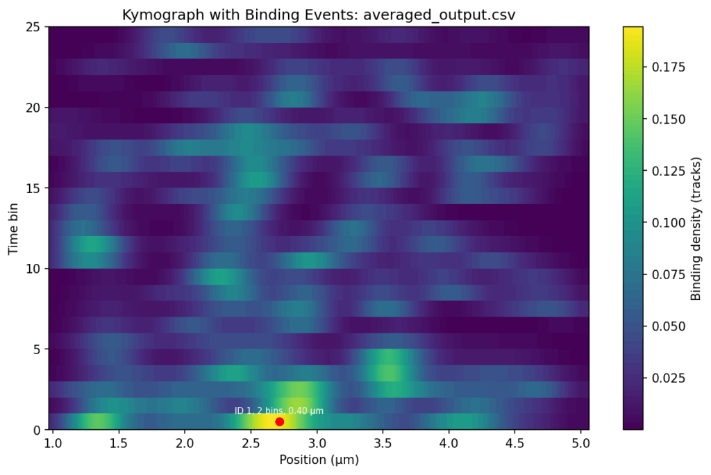
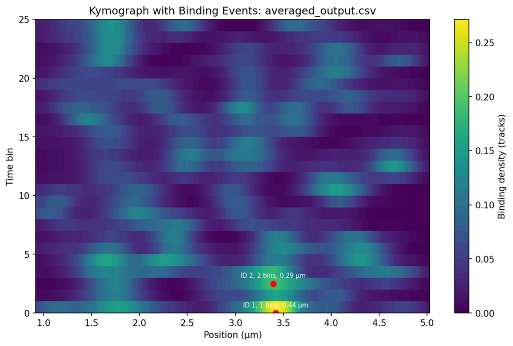
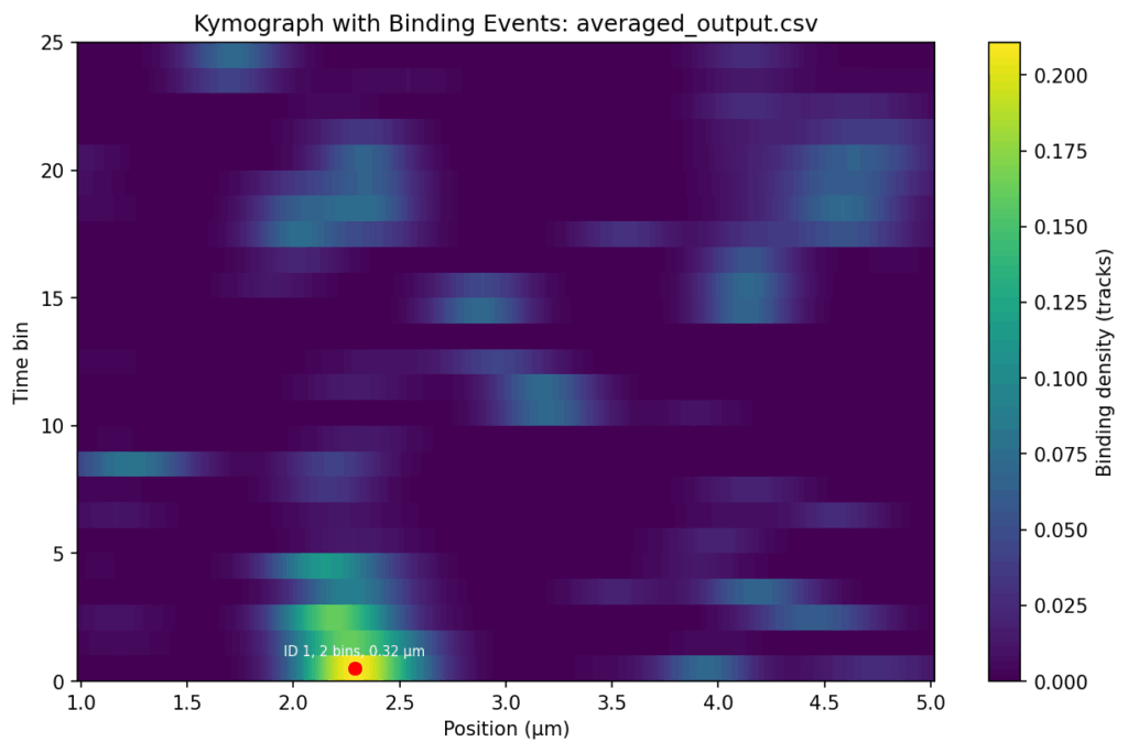
#2. Threshold-based detection: Apply a signal threshold (e.g., 0.16) to identify bound states at each position and time bin.
#3. Merging neighboring events: Combine adjacent bound regions in both position and time.
#4. Event filtering: Only merged events that satisfy the following conditions are reported as binding events and annotated in the plot:
* min_duration = 1 # minimum number of time bins
* min_range = 0.08 μm # minimum position spread for an event
5. Event statistics: Calculate time bin ranges, durations, peak sizes, and average positions for each event.
NEW_ADAPT: I have checked the files again, and those marked with 'my_...' are filtered by position and time. I sent you the unfiltered files so that you could create the nice heat maps that you made. So everything is correct. Could you do me two more favours?
Firstly, would it be possible to send me the heat maps of the '..._averaged_output_events' without the red dot, ID, bins and position?
Secondly, would it be possible to have a similar binding intensity scale for all three samples?
#--> Done with the new python code. TODO: update the post in bioinformatics.cc.
Thirdly, could you create the same heat maps, but with only the tracks above 5 seconds? That would be great.
#Solution for 3rd point: delete the input files the second columns for "ignoring the first time bin (namely time bin 0). "
#Additionally: delete the column "duration_bins" in averaged_output_events.csv and convert csv to Excel-file using csv2xls; TODO: observe in the new output Excel-files, the start_bin and end_bin, the numbers will be changed?
-
Used python scripts
- ~/DATA/Data_Vero_Kymographs/Vero_Lakeview/1_filter_track.py
- ~/DATA/Data_Vero_Kymographs/Vero_Lakeview/lake_files/2_generate_orig_lake_files.py
- ~/DATA/Data_Vero_Kymographs/Vero_Lakeview/3_update_lake.py
- ~/DATA/Data_Vero_Kymographs/Vero_Lakeview/4_merge_lake_files.py
- ~/DATA/Data_Vero_Kymographs/Binding_positions/overlap_v16_calculate_average_matix.py (Deprecated)
- ~/DATA/Data_Vero_Kymographs/Binding_positions/overlap_v17_draw_plot.py (Deprecated)
- python 1_combine_kymographs.py
- python 2_summarize_binding_events.py
-
Source code of 1_combine_kymographs.py
import pandas as pd
import numpy as np
import matplotlib.pyplot as plt
import glob
import os
from scipy.ndimage import label

# List of input CSV files
file_list = glob.glob("tracks_p853_250706_p502/*_binding_position_blue_filtered.csv")
#file_list = glob.glob("tracks_p853_250706_p502_averaged/averaged_output.csv")
#file_list = glob.glob("tracks_p853_250706_p502_sum/sum_output.csv")
print(f"Found {len(file_list)} CSV files: {file_list}")

# Ensure output directory exists
output_dir = os.path.dirname(file_list[0]) if file_list else "."
if not os.path.exists(output_dir):
    os.makedirs(output_dir)

# Collect all data
all_data = []
all_positions = []
for file in file_list:
    try:
        df = pd.read_csv(file, sep=';').rename(columns=lambda x: x.replace('# ', ''))
        positions = df['position (μm)'].values
        time_bins = df.columns[1:].values
        time_bin_data = df[df.columns[1:]].values
        all_positions.append(positions)
        all_data.append(time_bin_data)
    except Exception as e:
        print(f"Error processing {file} for data collection: {e}")
        continue

# Determine common position range and interpolate
min_pos = np.min([pos.min() for pos in all_positions if len(pos) > 0])
max_pos = np.max([pos.max() for pos in all_positions if len(pos) > 0])
max_len = max(len(pos) for pos in all_positions if len(pos) > 0)
common_positions = np.linspace(min_pos, max_pos, max_len)

# Interpolate each file's data
interpolated_data = []
for positions, time_bin_data in zip(all_positions, all_data):
    if len(positions) != time_bin_data.shape[0]:
        print("Warning: Mismatch in dimensions, skipping interpolation.")
        continue
    interpolated = np.zeros((time_bin_data.shape[1], len(common_positions)))
    for i in range(time_bin_data.shape[1]):
        interpolated[i] = np.interp(common_positions, positions, time_bin_data[:, i])
    interpolated_data.append(interpolated)

# Compute averaged data
if interpolated_data:
    averaged_data = np.mean(interpolated_data, axis=0)
else:
    print("No data available for averaging.")
    exit()

# Save averaged CSV
output_df = pd.DataFrame(averaged_data.T, columns=[f"time bin {i}" for i in range(averaged_data.shape[0])])
output_df.insert(0, 'position (μm)', common_positions)
output_csv_path = os.path.join(output_dir, 'averaged_output.csv')
output_df.to_csv(output_csv_path, sep=';', index=False)
print(f"Saved averaged output to {output_csv_path}")

# Compute summed data
if interpolated_data:
    sum_data = np.sum(interpolated_data, axis=0)
else:
    print("No data available for summing.")
    exit()

# Save summed CSV
output_df = pd.DataFrame(sum_data.T, columns=[f"time bin {i}" for i in range(sum_data.shape[0])])
output_df.insert(0, 'position (μm)', common_positions)
output_csv_path = os.path.join(output_dir, 'sum_output.csv')
output_df.to_csv(output_csv_path, sep=';', index=False)
print(f"Saved summed output to {output_csv_path}")

def plot_combined_kymograph(matrix, positions, output_dir, filename, title="Combined Kymograph"):
    """
    Plot combined kymograph for either averaged or summed data.

    Parameters
    ----------
    matrix : np.ndarray
        2D array of shape (num_time_bins, num_positions)
    positions : np.ndarray
        1D array of position coordinates
    output_dir : str
        Directory to save the plot
    filename : str
        Name of the output PNG file
    title : str
        Plot title
    """
    if matrix.size == 0:
        print("Empty matrix, skipping plot.")
        return

    plt.figure(figsize=(10, 6))
    max_ptp = np.max([np.ptp(line) for line in matrix]) if matrix.size > 0 else 1
    padding = 0.1 * np.max(matrix) if np.max(matrix) > 0 else 1
    offset_step = max_ptp + padding
    num_bins = matrix.shape[0]

    for i in range(num_bins):
        line = matrix[i]
        offset = i * offset_step
        plt.plot(positions, line + offset, 'b-', linewidth=0.5)

    y_ticks = [i * offset_step for i in range(num_bins)]
    y_labels = [f"time bin {i}" for i in range(num_bins)]
    plt.yticks(y_ticks, y_labels)
    plt.xlabel('Position (μm)')
    plt.ylabel('Binding Density')
    plt.title(title)

    output_path = os.path.join(output_dir, filename)
    plt.savefig(output_path, facecolor='white', edgecolor='none')
    plt.close()
    print(f"Saved combined kymograph plot to {output_path}")

# =============================
# Example usage
# =============================
# Plot averaged matrix
plot_combined_kymograph(averaged_data, common_positions, output_dir, 'combined_average_kymograph.png',
                        title="Averaged Binding Density Across All Files")

# Plot summed matrix
plot_combined_kymograph(sum_data, common_positions, output_dir, 'combined_sum_kymograph.png',
                        title="Summed Binding Density Across All Files")

# ======================================================
# Binding Event Detection + Plotting
# ======================================================

#signal_threshold = 0.2   # min photon density
#min_duration = 1         # min time bins
#min_range = 0.1         # μm, min position spread for an event
signal_threshold = 0.16   # min photon density
min_duration = 1         # min time bins
min_range = 0.08         # μm, min position spread for an event

for file in file_list:
    try:
        df = pd.read_csv(file, sep=';').rename(columns=lambda x: x.replace('# ', ''))
        positions = df['position (μm)'].values
        time_bins = df.columns[1:]
        photons_matrix = df[time_bins].values

        # Step 1: Binary mask
        mask = photons_matrix > signal_threshold

        # Step 2: Connected components
        labeled, num_features = label(mask, structure=np.ones((3, 3)))

        events = []
        for i in range(1, num_features + 1):
            coords = np.argwhere(labeled == i)
            pos_idx = coords[:, 0]
            time_idx = coords[:, 1]

            start_bin = time_idx.min()
            end_bin = time_idx.max()
            duration = end_bin - start_bin + 1

            pos_range = positions[pos_idx].max() - positions[pos_idx].min()

            # Apply filters
            if duration < min_duration or pos_range < min_range:
                continue

            avg_pos = positions[pos_idx].mean()
            peak_size = photons_matrix[pos_idx, time_idx].max()

            events.append({
                "start_bin": int(start_bin),
                "end_bin": int(end_bin),
                "duration_bins": int(duration),
                "pos_range": float(pos_range),
                "avg_position": float(avg_pos),
                "peak_size": float(peak_size)
            })

        # Print results
        print(f"\nBinding events for {os.path.basename(file)}:")
        if not events:
            print("No binding events detected.")
        else:
            for ev in events:
                print(
                    f" - Time bins {ev['start_bin']}–{ev['end_bin']} "
                    f"(duration {ev['duration_bins']}), "
                    f"Pos range: {ev['pos_range']:.2f} μm, "
                    f"Peak: {ev['peak_size']:.2f}, "
                    f"Avg pos: {ev['avg_position']:.2f} μm"
                )

        # Plot heatmap with detected events
        plt.figure(figsize=(10, 6))
        plt.imshow(
            photons_matrix.T,
            aspect='auto',
            origin='lower',
            extent=[positions.min(), positions.max(), 0, len(time_bins)],
            cmap='viridis'
        )
        plt.colorbar(label="Binding density (tracks)")  #Photon counts
        plt.xlabel("Position (μm)")
        plt.ylabel("Time bin")
        plt.title(f"Kymograph with Binding Events: {os.path.basename(file)}")

        # Annotate events on plot
        #for ev in events:
        #    mid_bin = (ev["start_bin"] + ev["end_bin"]) / 2
        #    plt.scatter(ev["avg_position"], mid_bin, color="red", marker="o", s=40)
        #    plt.text(
        #        ev["avg_position"], mid_bin + 0.5,
        #        f"{ev['duration_bins']} bins, {ev['pos_range']:.2f} μm",
        #        color="white", fontsize=7, ha="center"
        #    )

        out_path = os.path.join(output_dir, os.path.basename(file).replace(".csv", "_events.png"))
        plt.savefig(out_path, dpi=150, bbox_inches="tight")
        plt.close()
        print(f"Saved event plot to {out_path}")

    except Exception as e:
        print(f"Error processing {file}: {e}")
        continue
- Source code of 2_summarize_binding_events.py
import pandas as pd
import glob
import os
import argparse

# =============================
# Command-line arguments
# =============================
parser = argparse.ArgumentParser(description="Summarize binding-event CSV files in a folder.")
parser.add_argument("input_dir", type=str, help="Input directory containing CSV files")
args = parser.parse_args()
input_dir = args.input_dir

# =============================
# Prepare file list and output
# =============================
file_list = glob.glob(os.path.join(input_dir, "*.csv"))
print(f"Found {len(file_list)} CSV files in {input_dir}")

output_dir = "summaries"
os.makedirs(output_dir, exist_ok=True)

# Excel writer
excel_path = os.path.join(output_dir, "summary_all.xlsx")
with pd.ExcelWriter(excel_path, engine="xlsxwriter") as writer:

    for file in file_list:
        try:
            # Load CSV (ignore header lines with "#")
            df = pd.read_csv(file, sep=";", comment="#", header=None)

            # Assign proper column names
            df.columns = [
                "track index",
                "time (pixels)",
                "coordinate (pixels)",
                "time (seconds)",
                "position (um)",
                "minimum observable duration (seconds)"
            ]

            # Group by track index
            summaries = []
            for track, group in df.groupby("track index"):
                summary = {
                    "track index": track,
                    "n_events": len(group),
                    "time_start_s": round(group["time (seconds)"].min(), 3),
                    "time_end_s": round(group["time (seconds)"].max(), 3),
                    "duration_s": round(group["time (seconds)"].max() - group["time (seconds)"].min(), 3),
                    "pos_min_um": round(group["position (um)"].min(), 3),
                    "pos_max_um": round(group["position (um)"].max(), 3),
                    "pos_range_um": round(group["position (um)"].max() - group["position (um)"].min(), 3),
                    "pos_mean_um": round(group["position (um)"].mean(), 3)
                }
                summaries.append(summary)

            summary_df = pd.DataFrame(summaries)

            # Save each CSV summary individually
            out_csv_path = os.path.join(output_dir, os.path.basename(file).replace(".csv", "_summary.csv"))
            summary_df.to_csv(out_csv_path, sep=";", index=False, float_format="%.3f")
            print(f"Saved summary CSV for {file} -> {out_csv_path}")

            # Write summary to Excel sheet
            sheet_name = os.path.basename(file).replace(".csv", "")
            summary_df.to_excel(writer, sheet_name=sheet_name[:31], index=False, float_format="%.3f")

        except Exception as e:
            print(f"Error processing {file}: {e}")
            continue

print(f"Saved all summaries to Excel file -> {excel_path}")

