This article summarizes the pipeline and preserves all major code used for preparing metadata, processing raw counts, performing statistical analysis, integrating annotations, and reporting results. The workflow is designed for bacterial RNA-seq time-course analysis focusing on stress-related genes and oxidoreductases.
1. Prepare samples.tsv from the samplesheet
vim samples.tsvExample contents:
sample  condition   time_h  batch   genotype    medium  replicate
WT_MH_2h_1  WT_MH   2       WT  MH  1
WT_MH_2h_2  WT_MH   2       WT  MH  2
WT_MH_2h_3  WT_MH   2       WT  MH  3
WT_MH_4h_1  WT_MH   4       WT  MH  1
WT_MH_4h_2  WT_MH   4       WT  MH  2
WT_MH_4h_3  WT_MH   4       WT  MH  3
WT_MH_18h_1 WT_MH   18      WT  MH  1
WT_MH_18h_2 WT_MH   18      WT  MH  2
WT_MH_18h_3 WT_MH   18      WT  MH  3
deltasbp_MH_2h_1    deltasbp_MH 2       deltasbp    MH  1
deltasbp_MH_2h_2    deltasbp_MH 2       deltasbp    MH  2
deltasbp_MH_2h_3    deltasbp_MH 2       deltasbp    MH  3
...
deltasbp_TSB_18h_3  deltasbp_TSB    18      deltasbp    TSB 3
2. Reformat counts.tsv from STAR/Salmon
cp ./results/star_salmon/gene_raw_counts.csv counts.tsvClean file manually:
- Remove any double quotes (
"), removegene-from first column, replace delimiters to tab.
Clean file in R:
cts <- read.delim("counts.tsv", check.names = FALSE)
names(cts)[1] <- "gene_id"
if ("gene_name" %in% names(cts)) cts$gene_name <- NULL
names(cts) <- sub("_r([0-9]+)$", "_\\1", names(cts))
write.table(cts, file="counts_fixed.tsv", sep="\t", quote=FALSE, row.names=FALSE)
smp <- read.delim("samples.tsv", check.names = FALSE)
setdiff(colnames(cts)[-1], smp$sample)
setdiff(smp$sample, colnames(cts)[-1])
3. Run the R time-course analysis
Rscript rna_timecourse_bacteria.R \
  --counts counts_fixed.tsv \
  --samples samples.tsv \
  --condition_col condition \
  --time_col time_h \
  --emapper ~/DATA/Data_Michelle_RNAseq_2025/eggnog_out.emapper.annotations.txt \
  --volcano_csvs contrasts/ctrl_vs_treat.csv \
  --outdir results_bacteria
4. Summarize and convert results
~/Tools/csv2xls-0.4/csv_to_xls.py oxidoreductases_time_trends.tsv stress_genes_time_trends.tsv -d$'\t' -o oxidoreductases_and_stress_genes_time_trends.xls5. Key summary and reporting
PCA plots, time trends, and top decreasing/increasing genes by condition are summarized.
For further filtering, decreasing genes can be extracted by filtering direction == "decreasing" in the results tables.
6. Full main R script: rna_timecourse_bacteria.R
#!/usr/bin/env Rscript
# ===============================
# RNA-seq time-course helper (Bacteria) — DESeq2
# Uses eggNOG emapper annotations (GOs & EC) for oxidoreductases + stress genes
# ===============================
# Example:
# Rscript rna_timecourse_bacteria.R \
# --counts counts.tsv \
# --samples samples.tsv \
# --condition_col condition \
# --time_col time_h \
# --batch_col batch \
# --emapper ~/DATA/Data_Michelle_RNAseq_2025/eggnog_out.emapper.annotations.txt \
# --volcano_csvs contrasts/ctrl_vs_treat.csv \
# --outdir results_bacteria
#
# Assumptions:
# - counts.tsv: first column gene_id matching 'query' in emapper file
# - samples.tsv: columns 'sample', condition/time (numeric), optional batch
#
suppressPackageStartupMessages({
library(optparse)
library(DESeq2)
library(dplyr)
library(tidyr)
library(readr)
library(stringr)
library(ComplexHeatmap)
library(circlize)
library(ggplot2)
library(purrr)
})
opt_list <- list(
make_option("--counts", type="character", help="Counts matrix TSV (genes x samples). First col = gene_id"),
make_option("--samples", type="character", help="Sample metadata TSV with 'sample' column."),
make_option("--gene_id_col", type="character", default="gene_id", help="Counts gene id column name."),
make_option("--condition_col", type="character", default="condition", help="Condition column in samples."),
make_option("--time_col", type="character", default="time", help="Numeric time column in samples."),
make_option("--batch_col", type="character", default=NULL, help="Optional batch column."),
make_option("--emapper", type="character", help="eggNOG emapper annotations file (tab-delimited)."),
make_option("--volcano_csvs", type="character", default=NULL, help="Comma-separated volcano CSV/TSV files (must have a 'gene' column)."),
make_option("--outdir", type="character", default="results_bacteria", help="Output directory.")
)
opt <- parse_args(OptionParser(option_list = opt_list))
dir.create(opt$outdir, showWarnings = FALSE, recursive = TRUE)
message("[1/7] Load data")
counts <- read_tsv(opt$counts, col_types = cols())
stopifnot(opt$gene_id_col %in% colnames(counts))
counts <- as.data.frame(counts)
rownames(counts) <- counts[[opt$gene_id_col]]
counts[[opt$gene_id_col]] <- NULL
samples <- read_tsv(opt$samples, col_types = cols()) %>%
filter(sample %in% colnames(counts))
samples <- as.data.frame(samples)
rownames(samples) <- samples$sample
samples$sample <- NULL
samples[[opt$time_col]] <- as.numeric(samples[[opt$time_col]])
# --- Coerce counts to numeric and validate ---
# Remove any commas and coerce to numeric
counts[] <- lapply(counts, function(x) {
if (is.character(x)) x <- gsub(",", "", x, fixed = TRUE)
suppressWarnings(as.numeric(x))
})
# Report any NA introduced by coercion
na_cols <- vapply(counts, function(x) any(is.na(x)), logical(1))
if (any(na_cols)) {
bad <- names(which(na_cols))
message("WARNING: Non-numeric values detected in count columns; introduced NAs in: ", paste(bad, collapse=", "))
# Replace NA with 0 (safe fallback) and continue
counts[bad] <- lapply(counts[bad], function(x) { x[is.na(x)] <- 0; x })
}
# Ensure samples and counts columns align 1:1 and reorder counts accordingly
missing_in_samples <- setdiff(colnames(counts), rownames(samples))
missing_in_counts <- setdiff(rownames(samples), colnames(counts))
if (length(missing_in_samples) > 0) {
stop("These count columns have no matching row in samples.tsv: ", paste(missing_in_samples, collapse=", "))
}
if (length(missing_in_counts) > 0) {
stop("These samples.tsv rows have no matching column in counts.tsv: ", paste(missing_in_counts, collapse=", "))
}
counts <- counts[, rownames(samples), drop=FALSE]
# Finally, round to integers as required by DESeq2
counts <- round(as.matrix(counts))
message("[2/7] DESeq2 model (time-course)")
design_terms <- c()
if (!is.null(opt$batch_col) && opt$batch_col %in% colnames(samples)) {
design_terms <- c(design_terms, opt$batch_col)
}
design_terms <- c(design_terms, opt$condition_col, opt$time_col, paste0(opt$condition_col, ":", opt$time_col))
design_formula <- as.formula(paste("~", paste(design_terms, collapse=" + ")))
dds <- DESeqDataSetFromMatrix(countData = round(as.matrix(counts)),
colData = samples,
design = design_formula)
dds <- dds[rowSums(counts(dds)) > 1, ]
dds <- DESeq(dds, test="LRT",
full = design_formula,
reduced = as.formula(paste("~", paste(setdiff(design_terms, paste0(opt$condition_col, ":", opt$time_col)), collapse=" + "))))
vsd <- vst(dds, blind=FALSE)
vsd_mat <- assay(vsd)
message("[3/7] Parse emapper for GO/EC (oxidoreductases & stress genes)")
stopifnot(!is.null(opt$emapper))
emap <- read_tsv(opt$emapper, comment = "#", col_types = cols(.default = "c"))
# Expecting columns: query, GOs, EC, Description, Preferred_name, etc.
emap <- emap %>%
transmute(gene = query,
GOs = ifelse(is.na(GOs), "", GOs),
EC = ifelse(is.na(EC), "", EC),
Description = ifelse(is.na(Description), "", Description),
Preferred_name = ifelse(is.na(Preferred_name), "", Preferred_name))
emap <- emap %>% distinct(gene, .keep_all = TRUE)
# Flags:
# 1) oxidoreductase: EC starts with "1." OR GO includes GO:0016491
is_ox_by_ec <- grepl("^1\\.", emap$EC)
is_ox_by_go <- grepl("\\bGO:0016491\\b", emap$GOs)
emap$is_oxidoreductase <- is_ox_by_ec | is_ox_by_go
# 2) stress-related: search for stress GO ids in GOs
stress_gos <- c("GO:0006950","GO:0033554","GO:0006979","GO:0006974","GO:0009408","GO:0009266") # response to stress; cellular response; oxidative stress; DNA damage; response to heat; response to starvation
re_pat <- paste(stress_gos, collapse="|")
emap$is_stress <- grepl(re_pat, emap$GOs)
write_tsv(emap, file.path(opt$outdir, "emapper_flags.tsv"))
message("[4/7] Per-gene time slopes within each condition")
cond_levels <- unique(samples[[opt$condition_col]])
slope_summaries <- list()
for (cond in cond_levels) {
sel <- samples[[opt$condition_col]] == cond
mat <- vsd_mat[, sel, drop=FALSE]
tvec <- samples[[opt$time_col]][sel]
slopes <- apply(mat, 1, function(y) {
fit <- try(lm(y ~ tvec), silent = TRUE)
if (inherits(fit, "try-error")) return(c(NA, NA))
co <- summary(fit)$coefficients
c(beta=unname(co["tvec","Estimate"]), p=unname(co["tvec","Pr(>|t|)"]))
})
slopes <- t(slopes)
df <- as.data.frame(slopes)
df$gene <- rownames(mat)
df$condition <- cond
slope_summaries[[cond]] <- df
}
# (keep whatever you have above this point unchanged)
slope_df <- bind_rows(slope_summaries) %>%
mutate(padj = p.adjust(p, method="BH")) %>%
relocate(gene, condition, beta, p, padj)
# ---- Robust join to emapper ----
# clean IDs: trim; strip version suffixes like ".1"
emap$gene <- trimws(emap$gene)
emap$gene_clean <- sub("\\.\\d+$", "", emap$gene)
slope_df$gene <- trimws(slope_df$gene)
slope_df$gene_clean <- sub("\\.\\d+$", "", slope_df$gene)
# join on cleaned key
slope_df <- slope_df %>%
dplyr::left_join(
emap %>% dplyr::select(gene_clean, GOs, EC, Description, Preferred_name,
is_oxidoreductase, is_stress),
by = "gene_clean"
)
# recompute flags from EC/GOs when missing
slope_df <- slope_df %>%
mutate(
is_oxidoreductase = ifelse(
is.na(is_oxidoreductase),
(!is.na(EC) & grepl("^1\\.", EC)) | (!is.na(GOs) & grepl("\\bGO:0016491\\b", GOs)),
is_oxidoreductase
),
is_stress = ifelse(
is.na(is_stress),
(!is.na(GOs) & grepl("GO:0006950|GO:0033554|GO:0006979|GO:0006974|GO:0009408|GO:0009266", GOs)),
is_stress
)
) %>%
dplyr::select(-gene_clean)
# write full slopes
readr::write_tsv(slope_df, file.path(opt$outdir, "time_slopes_by_condition.tsv"))
# summaries
ox_summary <- slope_df %>%
dplyr::filter(!is.na(is_oxidoreductase) & is_oxidoreductase) %>%
dplyr::mutate(direction = dplyr::case_when(
beta < 0 & padj < 0.05 ~ "decreasing",
beta > 0 & padj < 0.05 ~ "increasing",
TRUE ~ "ns"
)) %>%
dplyr::arrange(padj, beta)
readr::write_tsv(ox_summary, file.path(opt$outdir, "oxidoreductases_time_trends.tsv"))
stress_summary <- slope_df %>%
dplyr::filter(!is.na(is_stress) & is_stress) %>%
dplyr::mutate(direction = dplyr::case_when(
beta < 0 & padj < 0.05 ~ "decreasing",
beta > 0 & padj < 0.05 ~ "increasing",
TRUE ~ "ns"
)) %>%
dplyr::arrange(padj, beta)
readr::write_tsv(stress_summary, file.path(opt$outdir, "stress_genes_time_trends.tsv"))
message("[5/7] Heatmaps from volcano gene lists (plus per-gene)")
make_heatmap <- function(glist, tag, kmeans_rows=NA) {
sub <- vsd_mat[rownames(vsd_mat) %in% glist, , drop=FALSE]
if (nrow(sub) == 0) {
message("No overlap for ", tag)
return(invisible(NULL))
}
z <- t(scale(t(sub)))
ha_col <- HeatmapAnnotation(
df = data.frame(
condition = samples[[opt$condition_col]],
time = samples[[opt$time_col]]
)
)
png(file.path(opt$outdir, paste0("heatmap_", tag, ".png")), width=1400, height=1000, res=140)
print(Heatmap(z, name="z", top_annotation = ha_col,
clustering_distance_rows = "euclidean",
clustering_method_rows = "ward.D2",
show_row_names = FALSE, show_column_names = TRUE,
row_km = kmeans_rows))
dev.off()
}
make_single_gene_heatmaps <- function(glist, tag) {
for (g in glist) {
if (!(g %in% rownames(vsd_mat))) next
z <- t(scale(t(vsd_mat[g,,drop=FALSE])))
png(file.path(opt$outdir, paste0("heatmap_", tag, "_", g, ".png")), width=1200, height=400, res=150)
print(Heatmap(z, name="z", cluster_rows=FALSE, cluster_columns=FALSE,
show_row_names=TRUE, show_column_names=TRUE))
dev.off()
}
}
if (!is.null(opt$volcano_csvs) && nzchar(opt$volcano_csvs)) {
files <- str_split(opt$volcano_csvs, ",")[[1]] %>% trimws()
for (f in files) {
df <- tryCatch({
if (grepl("\\.tsv$", f, ignore.case = TRUE)) read_tsv(f, col_types=cols())
else read_csv(f, col_types=cols())
}, error=function(e) NULL)
if (is.null(df) || !("gene" %in% names(df))) next
genes <- df$gene %>% unique()
tag <- tools::file_path_sans_ext(basename(f))
make_heatmap(genes, tag, kmeans_rows = 4)
make_single_gene_heatmaps(genes, paste0(tag, "_single"))
}
}
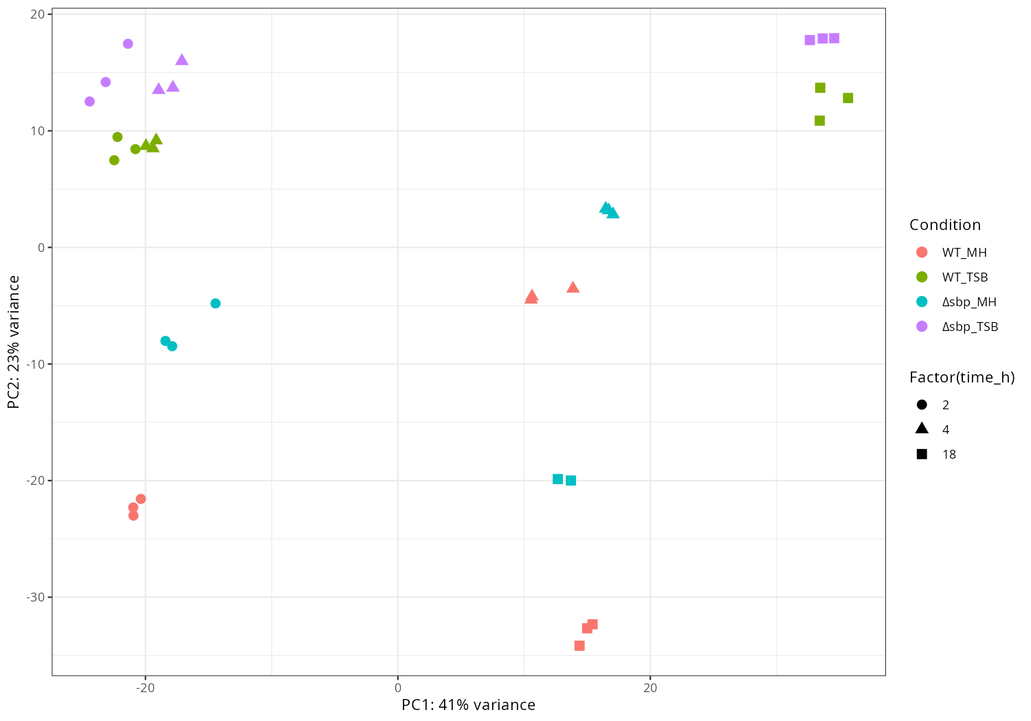
message("[6/7] PCA")
pca <- plotPCA(vsd, intgroup=c(opt$condition_col, opt$time_col), returnData = TRUE)
percentVar <- round(100 * attr(pca, "percentVar"))
# change 'deltasbp_*' to 'Δ_*' for legend labels
pca[[opt$condition_col]] <- gsub("^deltasbp", "Δsbp", pca[[opt$condition_col]])
p <- ggplot(pca, aes(PC1, PC2,
color = .data[[opt$condition_col]],
shape = factor(.data[[opt$time_col]]))) +
geom_point(size = 3) +
xlab(paste0("PC1: ", percentVar[1], "% variance")) +
ylab(paste0("PC2: ", percentVar[2], "% variance")) +
labs(color = "Condition", shape = "Factor(time_h)") + # legend titles
theme_bw()
ggsave(file.path(opt$outdir, "PCA_condition_time.png"), p, width=10, height=7, dpi=150)
message("[7/7] Summary")
summary_txt <- file.path(opt$outdir, "SUMMARY.txt")
sink(summary_txt)
cat("Bacterial time-course summary\n")
cat("Date:", as.character(Sys.time()), "\n\n")
cat("Conditions:", paste(unique(samples[[opt$condition_col]]), collapse=", "), "\n\n")
cat("Top oxidoreductases decreasing over time:\n")
print(ox_summary %>% filter(direction=="decreasing") %>% head(20))
cat("\nTop stress genes decreasing over time:\n")
print(stress_summary %>% filter(direction=="decreasing") %>% head(20))
sink()
message("Done -> ", opt$outdir)This code-rich summary provides a replicable basis for advanced bacterial RNA-seq time-course analysis and reporting. All main code steps and script logic are retained for transparency and practical reuse.